MLOps Blog

Brier Score: Understanding Model Calibration

Anass El Houd

6 min

29th August, 2023

ML Model Development

Do you ever encounter a storm when the probability of rain in your weather app is below 10%? Well, this shows perfectly how your plans can be destroyed with a not well-calibrated model (also known as an ill-calibrated model, or a model with a very high Brier score).

When building a prediction model, you take into account its predictive power by calculating different evaluation metrics. Some of them are common, like accuracy and precision. But others, like the Brier score in the weather forecasting model above, are often neglected.

In this tutorial you’ll get a simple, introductory explanation of Brier Score and calibration – one of the most important concepts used to evaluate prediction performance in statistics.

What is the Brier Score?

Brier Score evaluates the accuracy of probabilistic predictions.

Say we have two models that correctly predicted the sunny weather. One with the probability of 0.51 and the other with 0.93. They are both correct and have the same accuracy (assuming 0.5 threshold) but the second model feels better right? That is where Brier score comes in.

It is particularly useful when we are working with variables that can only take a finite number of values (we can call them categories or labels too).

For example, level of emergency (which takes four values: green, yellow, orange, and red), or whether tomorrow will be a rainy, cloudy or sunny day, or whether a threshold will be exceeded.

The Brier Score is more like a cost function. A lower value implies accurate predictions and vice versa. The primary goal of dealing with this concept is to decrease it.

The mathematical formulation of the Brier Score depends on the type of predicted variable. If we are developing a binary prediction, the score is given by:

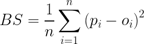
Where p is the prediction probability of occurrence of the event, and the term oi is equal to 1 if the event occurred and 0 if not.

Let’s take a very quick example to assimilate this concept. Let’s consider the event A=”Tomorrow is a sunny day”.

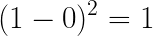
If you predict that the event A will occur with a probability of 100%, and the event occurs (the next is sunny which means o=1), the Brier score is equal to:

This is the lowest value possible. In other words: the best case we can achieve.

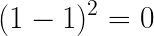
If we predicted the same event with the same probability, but the event doesn’t occur, the Brier score in this case is:

Say you predicted that the event A will occur with another probability, let’s say 60%. In case the event doesn’t occur in reality, the Brier Score will be:

As you may have noticed, the Brier score is a distance in the probability domain. Which means: the lower the value of this score, the better the prediction.

A perfect prediction will get a score of 0. The worst score is 1. It’s a synthetic criterion that provides combined information on the accuracy, robustness, and interpretability of the prediction model.

Dotted lines represent the worst cases (if the event occurs, the circle is equal to 1).

What is probability calibration?

Probability calibration is the post-processing of a model to improve its probability estimate. It helps us compare two models that have the same accuracy or other standard evaluation metrics.

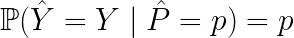
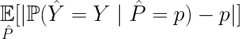
We say that a model is well calibrated when a prediction of a class with confidence p is correct 100p % of the time. To illustrate this calibration effect, let’s consider that you have a model that predicts cancer with a score of 70% for each patient out of 100. If your model is well calibrated, we would have 70 patients with cancer, if it is ill-calibrated, we will have more (or less). Therefore, the difference between these two models:

A model has an accuracy of 70% with 0.7 confidence in each prediction = well calibrated.
A model who has an accuracy of 70% with 0.9 confidence in each prediction = ill-calibrated.

For a perfect calibration, the relationship between the predicted probability and the fraction of positives follows the given:

The expression of this relationship is given by:

The figure above represents the reliability diagram of a model. We can plot it using scikit-learn as below:

import sklearn
from sklearn.calibration import calibration_curve
import matplotlib.lines as line
import matplotlib.pyplot as plt

x, y=calibration_curve(y_true, y_prob)

plt.plot(x,y)
ref = line.Line2D([0, 1], [0, 1], color='black')
transform = ax.transAxes
line.set_transform(transform)
ax.add_line(line)
fig.suptitle('Calibration – Neptune.ai')
ax.set_xlabel('Predicted probability')
ax.set_ylabel('Fraction of positive')
plt.legend()
plt.show()

Plotting the reliability curve for multiple models allows us to choose the best model not only based on its accuracy, but on its calibration too.

In the figure below, we can eliminate the SVC (0.163) model because it is far from being well calibrated.

calibration plots — *Figure taken from sklearn documentation*

If we want a numeric value to check the calibration of our models, we can use the calibration error given theoretically by:

When should you use the Brier score?

Evaluating the performance of a machine learning model is important, but it’s not enough to evaluate the real-world application predictions.

We often worry about:

the model’s confidence in its predictions,
its error distribution,
and how probability estimates are made.

In such cases, we need to use other performance factors. Brier score is an example.

This type of performance score is specifically used in high-risk applications. This score allows us to not treat the model results as real probabilities, but instead go beyond the raw results and check the model calibration, which is important for avoiding bad decision making or false interpretation.

Example of needing well-calibrated probabilities/model calibration

Let’s consider that you want to build a model that shows news pages to users by the chance of clicking on them. If the chance of the user clicking on a suggested item is high, the item is shown on the main page. Else, we show another item with a higher chance.

In this kind of problem, we don’t really care about how much the exact chance of clicking is, but only which item has the highest chance between all of the existing items. The model calibration is not really crucial here. What matters is which one of them has the highest probability (chance) of being clicked.

On the other hand, consider a problem in which we build a model that predicts the probability of contracting a specific disease based on the output of some analysis. The exact value of the probability is crucial here because it affects the decision of the doctor and the health of the patient.

Generally, calibration is used to improve a model when the results show that it has mistakes with high probabilities (or prediction score when the model doesn’t output the probability estimate e.g. random forest).

Of course, you can also look at other metrics that take prediction scores as input, like ROC AUC score, but they usually don’t focus on correctly calibrated probabilities. For example, ROC AUC focuses on ranking predictions.

Ok, now we can tell when the model is not well calibrated, but what can we do about it? How can we calibrate it?

Probability calibration methods

People use a lot of calibration methods. We will focus on the two most popular approaches:

Platt Scaling

Platt Scaling is often used to calibrate a model that we have already built. The principle of this method is based on the transformation of the outputs of our classification model into probability distribution.

Our model will not only give a categorical result (label or class), but also a degree of certainty about the result itself.

Instead of returning the class 1 as a result, it will return the probability of the correctness of this class prediction. Unfortunately, some classification models (like SVM) do not return probability values, or give poor probability estimates.

That’s why we use specific transformations to calibrate our model and convert the results into probability.

To use the Platt scaling method, we train our model normally, and then train the parameters of an additional sigmoid function to map the model outputs into probabilities.

You can do it using Logistic Regression fitted on the output of the model.

from sklearn.linear_model import LinearRegression

model=LinearRegression()
model.fit(p_out, y_out)
calib_p=model.predict(p_test)[:,1]

Isotonic Regression

Isotonic Regression does the same thing as Platt Scaling – they both transform model output into probability, and therefore calibrate it.

What’s the difference?

Platt Scaling uses a sigmoid shape to calibrate the model, which implies a sigmoid-shaped distortion in our probability distribution.

Isotonic Regression is a more powerful calibration method that can correct any monotonic distortion. It projects a non parametric function into a set of increasing functions (monotonic).

It is not recommended to use the isotonic regression if you have a small dataset, because it can easily overfit.

To implement this approach, we will again use sklearn (we assume you have already built and trained your “uncalibrated model”):

from sklearn.linear_model import IsotonicRegression

model=IsotonicRegression()
model.fit(p_out, y_out)
calib_p=model.transform(p_test)

Using model calibration on a real example

Let’s get some practice!

In order to keep it unique, we will generate two classes using make_classification from sklearn.

After that, we will train and fit an SVM classifier on the dataset.

from sklearn.datasets import make_classification
from sklearn.model_selection import train_test_split
from sklearn.svm import SVC

X, y = make_classification(n_samples=2500, n_classes=2)
X_train, X_test, y_train, y_test = train_test_split(X, y, test_size = 0.2)

We have just created our unique random data, and split it into a training set and test set.

Now we build the SVC Classifier, and fit it to the training set:

from sklearn.svm import SVC

svc_model=SVC()
svc_model.fit(X_train, y_train)

Let’s predict the results:

prob=svc_model.decision_function(X_test)

Next, let’s plot the calibration curve that we talked about earlier:

from sklearn.calibration import calibration_curve
x_p, y_p=calibration_curve(y_test, prob, n_bins=10, normalize=’True’)
plt.plot([0, 1], [0, 1])
plt.plot(x_p, y_p)
plt.show()

The result of the code above is the calibration curve or reliability curve:

This shows that our classifier is ill-calibrated (the calibration reference is the blue line).

Now let’s calculate the Brier score of this ill-calibrated model:

from sklearn.metrics import brier_score_loss, roc_auc_score

y_pred = svc_model.predict(X_test)
brier_score_loss(y_test, y_pred, pos_label=2)
roc_auc_score(y_test, y_pred)

For this, we get a ROC AUC score equal to 0,89 (means a good classification) and a Brief score equal to 0,49. Pretty high!

That explains the fact that the model is ill-calibrated. What do we do?

Let’s calibrate our model using sklearn again. We will apply Platt scaling (calibrate using sigmoid distribution). Sklearn offers a predefined function that does the job: CalibratedClassifierCV.

from sklearn.calibration import CalibratedClassifierCV
calib_model = CalibratedClassifierCV(svc_model, method='sigmoid', cv=5) calib_model.fit(X_train, y_train)
prob = calib_model.predict_proba(X_test)[:, 1]

#plot the calibration curve (see above to know what is it)
x_p, y_p = calibration_curve(y_test, prob, n_bins=10, normalize='True')
plt.plot([0, 1], [0, 1])
plt.plot(x_p, y_p)
plt.show()

The calibration or reliability curve of the model after calibration is shown below:

The reliability curve shows a tendency towards the calibration reference (the perfect case). For more verification, we can use the same numerical metrics as before.

In the following code, we calculate the Brier score and ROC AUC score of the calibrated model:

from sklearn.metrics import brier_score_loss, roc_auc_score

y_pred = calib_model.predict(X_test)
brier_score_loss(y_test, y_pred, pos_label=2)
roc_auc_score(y_test, y_pred)

The Brier score gets decreased after calibration (passed from 0,495 to 0,35), and we gain in terms of the ROC AUC score, which gets increased from 0,89 to 0,91.

We note that you may want to calibrate your model on a held-out set. In this case, we split the dataset to three parts:

We fit the model on the training set (first part).
We calibrate the model on the calibration set (second part).
We test the model on the testing set (third part).

Final thoughts

Calibrating your model is a crucial step to increase its prediction performance, especially if you care about “good” probability predictions that have a low Brier score.

However, you should keep in mind that it’s not obvious that improved calibrated probabilities will contribute to better predictions based on class or probability.

This potentially depends on the particular evaluation metric you use to test predictions. According to some papers, SVM, decision trees, and random forest are more likely to be improved after calibration (in our example we used a support vector classifier).

So as always proceed with caution.

I hope that, after reading this article you have a good understanding of what Brier score and model calibration are and you’ll be able to use that in your ML projects.

Thanks for reading!

References

[1] Brier GW. “Verification of forecasts expressed in terms of probability”. Mon Weather Rev 1950.
[2] Gneiting T, Raftery AE. “Strictly proper scoring rules, prediction, and estimation”. J Am Stat Assoc 2007.
[3] Is your model ready for the real world? – Inbar Naor – PyCon Israel Conference 2018
[4] A guide to calibration plots in Python – Chang Hsin Lee, February 2018.