How to Implement Customer Churn Prediction [Machine Learning Guide for Programmers]

When it comes to useful business applications of machine learning, it doesn’t get much better than customer churn prediction. It’s a problem where you usually have a lot of high-quality, fresh data to work with, it’s relatively straightforward, and solving it can be a great way to increase profits.

Churn rate is a critical metric of customer satisfaction. Low churn rates mean happy customers; high churn rates mean customers are leaving you. A small rate of monthly/quarterly churn compounds over time. 1% monthly churn quickly translates to almost 12% yearly churn. 

According to Forbes, it takes a lot more money (up to five times more) to get new customers than to keep the ones you already have. Churn tells you how many existing customers are leaving your business, so lowering churn has a big positive impact on your revenue streams.

Churn is a good indicator of growth potential. Churn rates track lost customers, and growth rates track new customers—comparing and analyzing both of these metrics tells you exactly how much your business is growing over time. If growth is higher than churn, you can say your business is growing. If churn is higher than growth, your business is getting smaller. 

In this article, we’re going to explore the churn rate in-depth and do an example implementation of a machine learning churn rate prediction system.

What is the churn rate?

Wikipedia states that the churn rate (also called attrition rate) measures the number of individuals or items moving out of a collective group over a specific period. It applies in many contexts, but the mainstream understanding of churn rate is related to the business case of customers that stop buying from you.

Software as a service (SaaS) with its subscription-based business model and membership-based businesses are at the forefront of innovative customer retention strategies. Analyzing growth in this space might involve tracking metrics (like revenues, new customer ratio, etc.), performing customer segmentation analysis, and predicting lifetime value. The churn rate is an input of customer lifetime value modeling that guides the estimation of net profit contributed to the whole future relationship with a customer. Independently, it calculates the percentage of discontinuity in subscriptions by customers of a service or product within a given time frame. 

This translates to revenue loss via customer cancellation. Market saturation is quite evident in the SaaS market, there are always plenty of alternatives for any SaaS product. Studying the churn rate can help with Knowing-Your-Customer (KYC) and effective retention and marketing strategies for subscription-driven businesses. 

Jeff Bezos once said, “We see our customers as guests to a party, and we are the hosts. It’s our job every day to make every important aspect of the customer experience a little bit better“. Improving customer retention is a continuous process, and understanding churn rate is the first step in the right direction.

You can classify churn as:

1. Customer and revenue churn
2. Voluntary and involuntary churn

Customer and revenue churn: Customer churn is simply the rate at which customers cancel their subscriptions. Also known as subscriber churn or logo churn, its value is represented in percentages. On the other hand, revenue churn is the loss in your monthly recurring revenue (MRR) at the beginning of the month. Customer churn and revenue churn aren’t always the same. You might have no customer churn, but still have revenue churn if customers are downgrading subscriptions. Negative churn is an ideal situation that only applies to revenue churn. The amount of new revenue from your existing customers (through cross-sells, upsells, and new signups) is more than the revenue you lose from cancellations and downgrades.

Voluntary and involuntary Churn: Voluntary churn is when the customer decides to cancel and takes the necessary steps to exit the service. It could be caused by dissatisfaction, or not receiving the value they expected. Involuntary churn happens due to situations such as expired payment details, server errors, insufficient funds, and other unpredictable predicaments. 

Customer satisfaction, happiness, and loyalty can be achieved to a certain degree, but churn will always be a part of the business. Churn can happen because of:

• Bad customer service (poor service quality, response rate, or overall customer experience),
• Finance issues (fees and rates),
• Customer needs change,
• Dissatisfaction (your service failed to meet expectations),
• Customers don’t see the value, 
• Customers switch to competitors,
• Long-time customers don’t feel appreciated.

0% churn rate is impossible. The trick is to keep the churn rate as low as possible at all times.

Importance of customer churn prediction

The impact of the churn rate is clear, so we need strategies to reduce it. Predicting churn is a good way to create proactive marketing campaigns targeted at the customers that are about to churn. 

Thanks to big data, forecasting customer churn with the help of machine learning is possible. Machine learning and data analysis are powerful ways to identify and predict churn. During churn prediction, you’re also:

• Identifying at-risk customers,
• Identifying customer pain points,
• Identifying strategy/methods to lower churn and increase customer retention.

Challenges of building an effective churn model

Here are the main challenges that might make it difficult for you to build an effective churn model:

• Inaccurate or messy customer data,
• Weak attrition exploratory analysis,
• Lack of information and domain knowledge,
• Lack of a coherent selection of a suitable churn modeling approach,
• Choice of metrics to validate churn model performance,
• Line of business (LoB) of services or products,
• Churn event censorship,
• Concept drift based on changes in customers behaviour patterns driving churn,
• Imbalance data (class imbalance issue).

Read also

How to Deal With Imbalanced Classification and Regression Data

Churn prediction use cases

Customer churn prediction is different based on the company’s line of business (LoB), operation workflow, and data architecture. The prediction model and application have to be tailored to the company’s needs, goals, and expectations. Some use cases for churn prediction are in:

• Telecommunication (cable or wireless network segment),
• Software as a service provider (SaaS),
• Retail market,
• Subscription-based businesses (media, music and video streaming services, etc.),
• Financial institutions (banking, insurance companies, Mortgage Companies, etc.),
• Marketing,
• Human Resource Management (Employee turnover).

Designing churn prediction workflow

The overall scope to build an ML-powered application to forecast customer churn is generic to standardized ML project structure that includes the following steps:

1. Defining problem and goal: It’s essential to understand what insights you need to get from the analysis and prediction. Understand the problem and collect requirements, stakeholder pain points, and expectations.
2. Establishing data source: Next, specify data sources that will be necessary for the modeling stage. Some popular sources of churn data are CRM systems, analytics services, and customer feedback.
3. Data preparation, exploration, and preprocessing: Raw historical data for solving the problem and building predictive models needs to be transformed into a format suitable for machine learning algorithms. This step can also improve overall results by increasing the quality of data.
4. Modeling and testing: This covers the development and performance validation of customers churn prediction models with various machine learning algorithms.
5. Deployment and monitoring: This is the last stage in applying machine learning for churn rate prediction. Here, the most suitable model is sent into production. It can be either integrated into existing software, or become the core of a newly built application.

Check also

The Life Cycle of a Machine Learning Project: What Are the Stages?

Deep dive: Telecom churn prediction system use case

The churn rate is very important in the telecommunications industry (wireless and cable service providers, satellite television providers, internet providers, etc). The churn rate in this use case provides clarity on the quality of the business, shows customer satisfaction with the product or service, and allows for comparison with competitors to gauge an acceptable level of churn. 

About the dataset

The sample data tracks a fictional telecommunications company, Telco. It’s customer churn data sourced by the IBM Developer Platform, and it’s available here. It includes a target label indicating whether or not the customer left within the last month, and other dependent features that cover demographics, services that each customer has signed up for, and customer account information. It has data for 7043 clients, with 20 features.

You can find this entire project on my Github.

Exploratory data analysis (EDA) 

Let’s critically explore the data to discover patterns and visualize how the features interact with the label (Churn or not).

Read also

Exploratory Data Analysis for Natural Language Processing: A Complete Guide to Python Tools

Let’s first import libraries for EDA, load the data, and print the first five rows:

#Import libraries
import numpy as np # linear algebra
import pandas as pd # data processing, CSV file I/O (e.g. pd.read_csv)
pd.set_option('display.max_columns', None)

import plotly.express as px #for visualization
import matplotlib.pyplot as plt #for visualization 

#Read the dataset
data_df = pd.read_csv("../data/churn.csv")

#Get overview of the data
def dataoveriew(df, message):
    print(f'{message}:n')
    print('Number of rows: ', df.shape[0])
    print("nNumber of features:", df.shape[1])
    print("nData Features:")
    print(df.columns.tolist())
    print("nMissing values:", df.isnull().sum().values.sum())
    print("nUnique values:")
    print(df.nunique())

dataoveriew(data_df, 'Overview of the dataset')

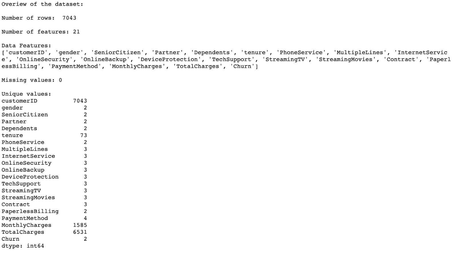
The dataset has 7043 rows and 21 columns. 

There are 17 categorical features:

• CustomerID: Customer ID unique for each customer
• gender: Whether the customer is a male or a female
• SeniorCitizen: Whether the customer is a senior citizen or not (1, 0)
• Partner: Whether the customer has a partner or not (Yes, No)
• Dependent: Whether the customer has dependents or not (Yes, No)
• PhoneService: Whether the customer has a phone service or not (Yes, No)
• MultipeLines: Whether the customer has multiple lines or not (Yes, No, No phone service)
• InternetService: Customer’s internet service provider (DSL, Fiber optic, No)
• OnlineSecurity: Whether the customer has online security or not (Yes, No, No internet service)
• OnlineBackup: Whether the customer has an online backup or not (Yes, No, No internet service)
• DeviceProtection: Whether the customer has device protection or not (Yes, No, No internet service)
• TechSupport: Whether the customer has tech support or not (Yes, No, No internet service)
• StreamingTV: Whether the customer has streaming TV or not (Yes, No, No internet service)
• StreamingMovies: Whether the customer has streaming movies or not (Yes, No, No internet service)
• Contract: The contract term of the customer (Month-to-month, One year, Two years)
• PaperlessBilling: The contract term of the customer (Month-to-month, One year, Two years)
• PaymentMethod: The customer’s payment method (Electronic check, Mailed check, Bank transfer (automatic), Credit card (automatic))

Next, there are 3 numerical features:

• Tenure: Number of months the customer has stayed with the company
• MonthlyCharges: The amount charged to the customer monthly
• TotalCharges: The total amount charged to the customer

Finally, there’s a prediction feature:

• Churn: Whether the customer churned or not (Yes or No)

These features can also be subdivided into:

• Demographic customer information:
  • gender , SeniorCitizen , Partner , Dependents
• Services that each customer has signed up for:
  • PhoneService , MultipleLines , InternetService , OnlineSecurity , OnlineBackup , DeviceProtection , TechSupport , StreamingTV , StreamingMovies,
• Customer account information:
  • tenure , Contract , PaperlessBilling , PaymentMethod , MonthlyCharges , TotalCharges

Let’s explore the target variable.

target_instance = data_df["Churn"].value_counts().to_frame()
target_instance = target_instance.reset_index()
target_instance = target_instance.rename(columns={'index': 'Category'})
fig = px.pie(target_instance, values='Churn', names='Category', color_discrete_sequence=["green", "red"],
             title='Distribution of Churn')
fig.show()

We’re trying to predict users that left the company in the previous month. It’s a binary classification problem with an unbalanced target.

• Churn: No – 73.5%
• Churn: Yes – 26.5%

Let’s explore categorical features.

#Defining bar chart function
def bar(feature, df=data_df ):
    #Groupby the categorical feature
    temp_df = df.groupby([feature, 'Churn']).size().reset_index()
    temp_df = temp_df.rename(columns={0:'Count'})
    #Calculate the value counts of each distribution and it's corresponding Percentages
    value_counts_df = df[feature].value_counts().to_frame().reset_index()
    categories = [cat[1][0] for cat in value_counts_df.iterrows()]
    #Calculate the value counts of each distribution and it's corresponding Percentages
    num_list = [num[1][1] for num in value_counts_df.iterrows()]
    div_list = [element / sum(num_list) for element in num_list]
    percentage = [round(element * 100,1) for element in div_list]
    #Defining string formatting for graph annotation
    #Numeric section
    def num_format(list_instance):
        formatted_str = ''
        for index,num in enumerate(list_instance):
            if index < len(list_instance)-2:
                formatted_str=formatted_str+f'{num}%, ' #append to empty string(formatted_str)
            elif index == len(list_instance)-2:
                formatted_str=formatted_str+f'{num}% & '
            else:
                formatted_str=formatted_str+f'{num}%'
        return formatted_str
    #Categorical section
    def str_format(list_instance):
        formatted_str = ''
        for index, cat in enumerate(list_instance):
            if index < len(list_instance)-2:
                formatted_str=formatted_str+f'{cat}, '
            elif index == len(list_instance)-2:
                formatted_str=formatted_str+f'{cat} & '
            else:
                formatted_str=formatted_str+f'{cat}'
        return formatted_str
    #Running the formatting functions
    num_str = num_format(percentage)
    cat_str = str_format(categories)

    #Setting graph framework
    fig = px.bar(temp_df, x=feature, y='Count', color='Churn', title=f'Churn rate by {feature}', barmode="group", color_discrete_sequence=["green", "red"])
    fig.add_annotation(
                text=f'Value count of distribution of {cat_str} are<br>{num_str} percentage respectively.',
                align='left',
                showarrow=False,
                xref='paper',
                yref='paper',
                x=1.4,
                y=1.3,
                bordercolor='black',
                borderwidth=1)
    fig.update_layout(
        # margin space for the annotations on the right
        margin=dict(r=400),
    )

    return fig.show()

Now, let’s plot the demographic features.

#Gender feature plot
bar('gender')
#SeniorCitizen feature plot 
data_df.loc[data_df.SeniorCitizen==0,'SeniorCitizen'] = "No"   #convert 0 to No in all data instances
data_df.loc[data_df.SeniorCitizen==1,'SeniorCitizen'] = "Yes"  #convert 1 to Yes in all data instances
bar('SeniorCitizen')
#Partner feature plot
bar('Partner')
#Dependents feature plot
bar('Dependents')

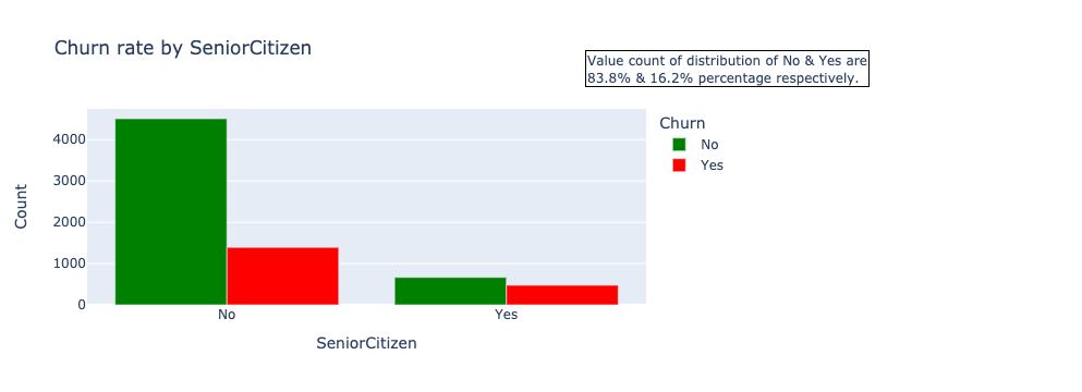
Demographic analysis insight: Gender and partner are evenly distributed with approximate percentage values. The difference in churn is slightly higher in females, but the small difference can be ignored. There’s a higher proportion of churn in younger customers (SeniorCitizen = No), customers with no partners, and customers with no dependents. The demographic section of data highlights on-senior citizens with no partners and dependents as a particular segment of customers likely to churn.

Next, let’s explore the services that each customer has signed up for.

bar('PhoneService')
bar('MultipleLines')
bar('InternetService')
bar('OnlineSecurity')
bar('OnlineBackup')
bar('DeviceProtection')
bar('TechSupport')
bar('StreamingTV')
bar('StreamingMovies')

Services that each customer has signed up for insight: These features show significant variations across their values. If a customer doesn’t have phone service, they can’t have multiple lines. About 90.3% of the customers have phone services and have a higher rate to churn. Customers who have fibre optic as an internet service are more likely to churn. This can happen due to high prices, competition, customer service, and many other reasons. Fiber optic service is much more expensive than DSL, which may be one of the reasons why customers churn. Customers with  OnlineSecurity, OnlineBackup, DeviceProtection, and TechSupport are more unlikely to churn. Streaming service is not predictive for churn as it’s evenly distributed to yes and no options.

Time to explore payment features.

bar('Contract')
bar('PaperlessBilling')
bar('PaymentMethod')

Payment insights: The shorter the contract, the higher the churn rate. Those with more extended plans face additional barriers when canceling early. This clearly explains the motivation for companies to have long-term relationships with their customers. Churn Rate is higher for the customers who opted for paperless billing. About 59.2% of customers use paperless billing. Customers who pay with electronic checks are more likely to churn, and this kind of payment is more common than other payment types.

Now, let’s explore numeric features.

Data_df.dtypes

It can be observed that the TotalCharges has an object data type which means that it contains string components. Let’s convert it.

# Let’s catch the error
try:
    data_df['TotalCharges'] = data_df['TotalCharges'].astype(float)
except ValueError as ve:
    print (ve)

This indicates that some empty values are stored as empty spaces. Let’s transform the feature into a numerical format while equating these empty string spaces as NaN as follows:

data_df['TotalCharges'] = pd.to_numeric(data_df['TotalCharges'],errors='coerce')
#Fill the missing values with with the median value
data_df['TotalCharges'] = data_df['TotalCharges'].fillna(data_df['TotalCharges'].median())

Next, let’s plot the histogram of all the numeric features to understand the distribution.

# Defining the histogram plotting function
def hist(feature):
    group_df = data_df.groupby([feature, 'Churn']).size().reset_index()
    group_df = group_df.rename(columns={0: 'Count'})
    fig = px.histogram(group_df, x=feature, y='Count', color='Churn', marginal='box', title=f'Churn rate frequency to {feature} distribution', color_discrete_sequence=["green", "red"])
    fig.show()

Running the functions on the numeric features as follows:

hist('tenure')
hist('MonthlyCharges')
hist('TotalCharges')

Customer account information insight: The tenure histogram is rightly skewed and shows that most customers have been with the telecom company for just the first few months (0-9 months). The highest rate of churn is also in the first few months (0-9months). 75% of customers who end up leaving the Telco company do so within their first 30 months. The monthly charge histogram shows that clients with higher monthly charges have a higher churn rate. This suggests that discounts and promotions can be an enticing reason for customers to stay.

Let’s bin the numeric features into three sections based on quantiles (low, medium, and high to get more information from it).

#Create an empty dataframe
bin_df = pd.DataFrame()

#Update the binning dataframe
bin_df['tenure_bins'] =  pd.qcut(data_df['tenure'], q=3, labels= ['low', 'medium', 'high'])
bin_df['MonthlyCharges_bins'] =  pd.qcut(data_df['MonthlyCharges'], q=3, labels= ['low', 'medium', 'high'])
bin_df['TotalCharges_bins'] =  pd.qcut(data_df['TotalCharges'], q=3, labels= ['low', 'medium', 'high'])
bin_df['Churn'] = data_df['Churn']

#Plot the bar chart of the binned variables
bar('tenure_bins', bin_df)
bar('MonthlyCharges_bins', bin_df)
bar('TotalCharges_bins', bin_df)

Based on binning, the low tenure and high monthly charge bins have higher churn rates, as supported by the previous analysis. At the same time, the low Total charge bin has a higher churn rate. 

Data preprocessing

In this section, we’ll gain more insights and convert the data into a data representation suitable for various machine learning algorithms.

# The customerID column isnt useful as the feature is used for identification of customers. 
data_df.drop(["customerID"],axis=1,inplace = True)

# Encode categorical features

#Defining the map function
def binary_map(feature):
    return feature.map({'Yes':1, 'No':0})

## Encoding target feature
data_df['Churn'] = data_df[['Churn']].apply(binary_map)

# Encoding gender category
data_df['gender'] = data_df['gender'].map({'Male':1, 'Female':0})

#Encoding other binary category
binary_list = ['SeniorCitizen', 'Partner', 'Dependents', 'PhoneService', 'PaperlessBilling']
data_df[binary_list] = data_df[binary_list].apply(binary_map)

#Encoding the other categoric features with more than two categories
data_df = pd.get_dummies(data_df, drop_first=True)

Check also

A Comprehensive Guide to Data Preprocessing

Let’s see the correlation between values.

# Checking the correlation between features
corr = data_df.corr()

fig = px.imshow(corr,width=1000, height=1000)
fig.show()

Correlation measures the linear relationship between two variables. Features with high correlation are more linearly dependent and have almost the same effect on the dependent variable. So, when two features have a high correlation, we can drop one of them. In our case, we can drop highly correlated features like MultipleLines, OnlineSecurity, OnlineBackup, DeviceProtection, TechSupport, StreamingTV, and StreamingMovies.

Churn prediction is a binary classification problem, as customers either churn or are retained in a given period. Two questions need answering to guide model building:

1. Which features make customers churn or retain?
2. What are the most important features to train a model with high performance?

Let’s use the generalized linear model (GLM) to gain some statistics of the respective features with the target.

import statsmodels.api as sm
import statsmodels.formula.api as smf

#Change variable name separators to '_'
all_columns = [column.replace(" ", "_").replace("(", "_").replace(")", "_").replace("-", "_") for column in data_df.columns]

#Effect the change to the dataframe column names
data_df.columns = all_columns

#Prepare it for the GLM formula
glm_columns = [e for e in all_columns if e not in ['customerID', 'Churn']]
glm_columns = ' + '.join(map(str, glm_columns))

#Fiting it to the Generalized Linear Model
glm_model = smf.glm(formula=f'Churn ~ {glm_columns}', data=data_df, family=sm.families.Binomial())
res = glm_model.fit()
print(res.summary())

For the first question, you should look at the (P>|z|) column. If the absolute p-value is smaller than 0.05, it means that the feature affects Churn in a statistically significant way. Examples are:

• SeniorCitizen
• Tenure
• Contract
• PaperlessBillings etc.

The second question about feature importances can be answered by looking at the exponential coefficient values. The exponential coefficient estimates the expected change in churn through a given feature by a change of one unit.

np.exp(res.params)

This outputs the odd ratios. Values more than 1 indicate increased churn. Values less than 1 indicate that churn is happening less.

The range of all features should be normalized so that each feature contributes approximately proportionately to the final distance, so we do feature scaling.

#feature scaling
from sklearn.preprocessing import MinMaxScaler
sc = MinMaxScaler()
data_df['tenure'] = sc.fit_transform(data_df[['tenure']])
data_df['MonthlyCharges'] = sc.fit_transform(data_df[['MonthlyCharges']])
data_df['TotalCharges'] = sc.fit_transform(data_df[['TotalCharges']])

Let’s start creating a baseline model with a Logistic Regression algorithm, then predict with other machine learning models like Support Vector Classifier (SVC), Random Forest Classifier, Decision-tree classifier, and Naive-Bayes Classifier.

# Import Machine learning algorithms
from sklearn.linear_model import LogisticRegression
from sklearn.svm import SVC
from sklearn.ensemble import RandomForestClassifier
from sklearn.tree import DecisionTreeClassifier
from sklearn.naive_bayes import GaussianNB

#Import metric for performance evaluation
from sklearn.metrics import accuracy_score, precision_score, recall_score, f1_score

#Split data into train and test sets
from sklearn.model_selection import train_test_split
X = data_df.drop('Churn', axis=1)
y = data_df['Churn']
X_train, X_test, y_train, y_test = train_test_split(X, y, test_size=0.3, random_state=50)

#Defining the modelling function
def modeling(alg, alg_name, params={}):
    model = alg(**params) #Instantiating the algorithm class and unpacking parameters if any
    model.fit(X_train, y_train)
    y_pred = model.predict(X_test)

    #Performance evaluation
    def print_scores(alg, y_true, y_pred):
        print(alg_name)
        acc_score = accuracy_score(y_true, y_pred)
        print("accuracy: ",acc_score)
        pre_score = precision_score(y_true, y_pred)
        print("precision: ",pre_score)
        rec_score = recall_score(y_true, y_pred)
        print("recall: ",rec_score)
        f_score = f1_score(y_true, y_pred, average='weighted')
        print("f1_score: ",f_score)

    print_scores(alg, y_test, y_pred)
    return model

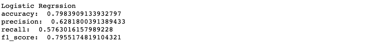
# Running logistic regression model
log_model = modeling(LogisticRegression, 'Logistic Regression')

Next, we do feature selection to enable the machine learning algorithm to train faster, reduce model complexity, increase interpretability, and improve model accuracy if the right features subset is chosen.

# Feature selection to improve model building
from sklearn.feature_selection import RFECV
from sklearn.model_selection import StratifiedKFold
log = LogisticRegression()
rfecv = RFECV(estimator=log, cv=StratifiedKFold(10, random_state=50, shuffle=True), scoring="accuracy")
rfecv.fit(X, y)

plt.figure(figsize=(8, 6))
plt.plot(range(1, len(rfecv.grid_scores_)+1), rfecv.grid_scores_)
plt.grid()
plt.xticks(range(1, X.shape[1]+1))
plt.xlabel("Number of Selected Features")
plt.ylabel("CV Score")
plt.title("Recursive Feature Elimination (RFE)")
plt.show()

print("The optimal number of features: {}".format(rfecv.n_features_))

#Saving dataframe with optimal features
X_rfe = X.iloc[:, rfecv.support_]

#Overview of the optimal features in comparison with the intial dataframe
print(""X" dimension: {}".format(X.shape))
print(""X" column list:", X.columns.tolist())
print(""X_rfe" dimension: {}".format(X_rfe.shape))
print(""X_rfe" column list:", X_rfe.columns.tolist())

<pre class="hljs" style="display: block; overflow-x: auto; padding: 0.5em; color: rgb(51, 51, 51); background: rgb(248, 248, 248);"><span class="hljs-comment" style="color: rgb(153, 153, 136); font-style: italic;"># Splitting data with optimal features</span>
X_train, X_test, y_train, y_test = train_test_split(X_rfe, y, test_size=<span class="hljs-number" style="color: teal;">0.3</span>, random_state=<span class="hljs-number" style="color: teal;">50</span>)

<span class="hljs-comment" style="color: rgb(153, 153, 136); font-style: italic;"># Running logistic regression model</span>
log_model = modeling(LogisticRegression, <span class="hljs-string" style="color: rgb(221, 17, 68);">'Logistic Regression Classification'</span>)
</pre>

### Trying other machine learning algorithms: SVC
svc_model = modeling(SVC, 'SVC Classification')

#Random forest
rf_model = modeling(RandomForestClassifier, "Random Forest Classification")

#Decision tree
dt_model = modeling(DecisionTreeClassifier, "Decision Tree Classification")

#Naive bayes 
nb_model = modeling(GaussianNB, "Naive Bayes Classification")

From the selected performance metrics, the Logistic Regression algorithm has the highest scores across all chosen metrics. It can be improved with various techniques, but we’ll quickly improve it with hyperparameter tuning (Random search).

## Improve best model by hyperparameter tuning
# define model
model = LogisticRegression()

# define evaluation
from sklearn.model_selection import RepeatedStratifiedKFold
cv = RepeatedStratifiedKFold(n_splits=10, n_repeats=3, random_state=1)

# define search space
from scipy.stats import loguniform
space = dict()
space['solver'] = ['newton-cg', 'lbfgs', 'liblinear']
space['penalty'] = ['none', 'l1', 'l2', 'elasticnet']
space['C'] = loguniform(1e-5, 1000)

# define search
from sklearn.model_selection import RandomizedSearchCV
search = RandomizedSearchCV(model, space, n_iter=500, scoring='accuracy', n_jobs=-1, cv=cv, random_state=1)

# execute search
result = search.fit(X_rfe, y)
# summarize result
# print('Best Score: %s' % result.best_score_)
# print('Best Hyperparameters: %s' % result.best_params_)
params = result.best_params_

#Improving the Logistic Regression model
log_model = modeling(LogisticRegression, 'Logistic Regression Classification', params=params)

The model improved slightly. Let’s save the model and start the deployment of our churn prediction application using this model.

#Saving best model 
import joblib
#Sava the model to disk
filename = 'model.sav'
joblib.dump(log_model, filename)

Deployment

It’s essential to deploy your model so that predictions can be made from a trained ML model available to others, whether users, management, or other systems. We’ll use Streamlit in this section. It’s an open-source Python library that makes it easy to create and share beautiful, custom web apps for machine learning and data science.

May interest you

Streamlit Guide: How to Build Machine Learning Applications
Best 8 Machine Learning Model Deployment Tools That You Need to Know

The application to be deployed will function via operational use cases:

1. Online prediction: This use case generates predictions on a one-by-one basis for each data point (in the context of this article, a customer).
2. Batch prediction: This use is for generating predictions for a set of observations instantaneously.

The deployment script is as follows:

#Import libraries
import streamlit as st
import pandas as pd
import numpy as np
from PIL import Image

#load the model from disk
import joblib
model = joblib.load(r"./notebook/model.sav")

#Import python scripts
from preprocessing import preprocess

def main():
    #Setting Application title
    st.title('Telco Customer Churn Prediction App')

      #Setting Application description
    st.markdown("""
     :dart:  This Streamlit app is made to predict customer churn in a ficitional telecommunication use case.
    The application is functional for both online prediction and batch data prediction. n
    """)
    st.markdown("<h3></h3>", unsafe_allow_html=True)

    #Setting Application sidebar default
    image = Image.open('App.jpg')
    add_selectbox = st.sidebar.selectbox(
    "How would you like to predict?", ("Online", "Batch"))
    st.sidebar.info('This app is created to predict Customer Churn')
    st.sidebar.image(image)

    if add_selectbox == "Online":
        st.info("Input data below")
        #Based on our optimal features selection
        st.subheader("Demographic data")
        seniorcitizen = st.selectbox('Senior Citizen:', ('Yes', 'No'))
        dependents = st.selectbox('Dependent:', ('Yes', 'No'))
        st.subheader("Payment data")
        tenure = st.slider('Number of months the customer has stayed with the company', min_value=0, max_value=72, value=0)
        contract = st.selectbox('Contract', ('Month-to-month', 'One year', 'Two year'))
        paperlessbilling = st.selectbox('Paperless Billing', ('Yes', 'No'))
        PaymentMethod = st.selectbox('PaymentMethod',('Electronic check', 'Mailed check', 'Bank transfer (automatic)','Credit card (automatic)'))
        monthlycharges = st.number_input('The amount charged to the customer monthly', min_value=0, max_value=150, value=0)
        totalcharges = st.number_input('The total amount charged to the customer',min_value=0, max_value=10000, value=0)

        st.subheader("Services signed up for")
        mutliplelines = st.selectbox("Does the customer have multiple lines",('Yes','No','No phone service'))
        phoneservice = st.selectbox('Phone Service:', ('Yes', 'No'))
        internetservice = st.selectbox("Does the customer have internet service", ('DSL', 'Fiber optic', 'No'))
        onlinesecurity = st.selectbox("Does the customer have online security",('Yes','No','No internet service'))
        onlinebackup = st.selectbox("Does the customer have online backup",('Yes','No','No internet service'))
        techsupport = st.selectbox("Does the customer have technology support", ('Yes','No','No internet service'))
        streamingtv = st.selectbox("Does the customer stream TV", ('Yes','No','No internet service'))
        streamingmovies = st.selectbox("Does the customer stream movies", ('Yes','No','No internet service'))

        data = {
                'SeniorCitizen': seniorcitizen,
                'Dependents': dependents,
                'tenure':tenure,
                'PhoneService': phoneservice,
                'MultipleLines': mutliplelines,
                'InternetService': internetservice,
                'OnlineSecurity': onlinesecurity,
                'OnlineBackup': onlinebackup,
                'TechSupport': techsupport,
                'StreamingTV': streamingtv,
                'StreamingMovies': streamingmovies,
                'Contract': contract,
                'PaperlessBilling': paperlessbilling,
                'PaymentMethod':PaymentMethod,
                'MonthlyCharges': monthlycharges,
                'TotalCharges': totalcharges
                }
        features_df = pd.DataFrame.from_dict([data])
        st.markdown("<h3></h3>", unsafe_allow_html=True)
        st.write('Overview of input is shown below')
        st.markdown("<h3></h3>", unsafe_allow_html=True)
        st.dataframe(features_df)
        #Preprocess inputs
        preprocess_df = preprocess(features_df, 'Online')

        prediction = model.predict(preprocess_df)

        if st.button('Predict'):
            if prediction == 1:
                st.warning('Yes, the customer will terminate the service.')
            else:
                st.success('No, the customer is happy with Telco Services.')


    else:
        st.subheader("Dataset upload")
        uploaded_file = st.file_uploader("Choose a file")
        if uploaded_file is not None:
            data = pd.read_csv(uploaded_file)
            #Get overview of data
            st.write(data.head())
            st.markdown("<h3></h3>", unsafe_allow_html=True)
            #Preprocess inputs
            preprocess_df = preprocess(data, "Batch")
            if st.button('Predict'):
                #Get batch prediction
                prediction = model.predict(preprocess_df)
                prediction_df = pd.DataFrame(prediction, columns=["Predictions"])
                prediction_df = prediction_df.replace({1:'Yes, the customer will terminate the service.',
                                                    0:'No, the customer is happy with Telco Services.'})

                st.markdown("<h3></h3>", unsafe_allow_html=True)
                st.subheader('Prediction')
                st.write(prediction_df)

if __name__ == '__main__':
        main()

The preprocessing script that was imported into the application script can be found in the project repo here.

Demo

Conclusion

Churn rate is an important indicator for subscription-based companies. Identifying customers who aren’t happy can help managers identify product or pricing plan weak points, operation issues, as well as customer preferences and expectations. When you know all that, it’s easier to introduce proactive ways of reducing churn.