Neptune Blog

Keras Loss Functions: Everything You Need to Know

Derrick Mwiti

6 min

22nd July, 2025

ML Model Development

You’ve created a deep learning model in Keras, you prepared the data and now you are wondering which loss you should choose for your problem.

We’ll get to that in a second but first what is a loss function?

In deep learning, the loss is computed to get the gradients with respect to model weights and update those weights accordingly via backpropagation. Loss is calculated and the network is updated after every iteration until model updates don’t bring any improvement in the desired evaluation metric.

So while you keep using the same evaluation metric like f1 score or AUC on the validation set during (long parts) of your machine learning project, the loss can be changed, adjusted and modified to get the best evaluation metric performance.

You can think of the loss function just like you think about the model architecture or the optimizer and it is important to put some thought into choosing it. In this piece we’ll look at:

loss functions available in Keras and how to use them,
how you can define your own custom loss function in Keras,
how to add sample weighing to create observation-sensitive losses,
how to avoid nans in the loss,
how you can monitor the loss function via plotting and callbacks.

Let’s get into it!

Keras loss functions 101

In Keras, loss functions are passed during the compile stage, as shown below.

In this example, we’re defining the loss function by creating an instance of the loss class. Using the class is advantageous because you can pass some additional parameters.

from tensorflow import keras
from tensorflow.keras import layers

model = keras.Sequential()
model.add(layers.Dense(64, kernel_initializer='uniform', input_shape=(10,)))
model.add(layers.Activation('softmax'))

loss_function = keras.losses.SparseCategoricalCrossentropy(from_logits=True)
model.compile(loss=loss_function, optimizer='adam')

If you want to use a loss function that is built into Keras without specifying any parameters you can just use the string alias as shown below:

model.compile(loss='sparse_categorical_crossentropy', optimizer='adam')

You might be wondering how does one decide on which loss function to use?

There are various loss functions available in Keras. Other times you might have to implement your own custom loss functions.

Let’s dive into all those scenarios.

Which loss functions are available in Keras?

Binary Classification

Binary classification loss function comes into play when solving a problem involving just two classes. For example, when predicting fraud in credit card transactions, a transaction is either fraudulent or not.

Binary Cross Entropy

The BinaryCrossentropy will calculate the cross-entropy loss between the predicted classes and the true classes. By default, the sum_over_batch_size reduction is used. This means that the loss will return the average of the per-sample losses in the batch.

y_true = [[0., 1.], [0.2, 0.8],[0.3, 0.7],[0.4, 0.6]]
y_pred = [[0.6, 0.4], [0.4, 0.6],[0.6, 0.4],[0.8, 0.2]]
bce = tf.keras.losses.BinaryCrossentropy(reduction='sum_over_batch_size')
bce(y_true, y_pred).numpy()

The sum reduction means that the loss function will return the sum of the per-sample losses in the batch.

bce = tf.keras.losses.BinaryCrossentropy(reduction='sum')
bce(y_true, y_pred).numpy()

Using the reduction as none returns the full array of the per-sample losses.

bce = tf.keras.losses.BinaryCrossentropy(reduction='none')
bce(y_true, y_pred).numpy()
array([0.9162905 , 0.5919184 , 0.79465103, 1.0549198 ], dtype=float32)

In binary classification, the activation function used is the sigmoid activation function. It constrains the output to a number between 0 and 1.

Multiclass classification

Problems involving the prediction of more than one class use different loss functions. In this section we’ll look at a couple:

Categorical Crossentropy

The CategoricalCrossentropy also computes the cross-entropy loss between the true classes and predicted classes. The labels are given in an one_hot format.

cce = tf.keras.losses.CategoricalCrossentropy()
cce(y_true, y_pred).numpy()

Sparse Categorical Crossentropy

If you have two or more classes and the labels are integers, the SparseCategoricalCrossentropy should be used.

y_true = [0, 1,2]
y_pred = [[0.05, 0.95, 0], [0.1, 0.8, 0.1],[0.1, 0.8, 0.1]]
scce = tf.keras.losses.SparseCategoricalCrossentropy()
scce(y_true, y_pred).numpy()

The Poison Loss

You can also use the Poisson class to compute the poison loss. It’s a great choice if your dataset comes from a Poisson distribution for example the number of calls a call center receives per hour.

y_true = [[0.1, 1.,0.8], [0.1, 0.9,0.1],[0.2, 0.7,0.1],[0.3, 0.1,0.6]]
y_pred = [[0.6, 0.2,0.2], [0.2, 0.6,0.2],[0.7, 0.1,0.2],[0.8, 0.1,0.1]]
p = tf.keras.losses.Poisson()
p(y_true, y_pred).numpy()

Kullback-Leibler Divergence Loss

The relative entropy can be computed using the KLDivergence class. According to the official docs at PyTorch:

KL divergence is a useful distance measure for continuous distributions and is often useful when performing direct regression over the space of (discretely sampled) continuous output distributions.

y_true = [[0.1, 1.,0.8], [0.1, 0.9,0.1],[0.2, 0.7,0.1],[0.3, 0.1,0.6]]
y_pred = [[0.6, 0.2,0.2], [0.2, 0.6,0.2],[0.7, 0.1,0.2],[0.8, 0.1,0.1]]
kl = tf.keras.losses.KLDivergence()
kl(y_true, y_pred).numpy()

In a multi-class problem, the activation function used is the softmax function.

Object Detection

The Focal Loss

In classification problems involving imbalanced data and object detection problems, you can use the Focal Loss. The loss introduces an adjustment to the cross-entropy criterion.

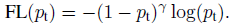
It is done by altering its shape in a way that the loss allocated to well-classified examples is down-weighted. This ensures that the model is able to learn equally from minority and majority classes.

The cross-entropy loss is scaled by scaling the factors decaying at zero as the confidence in the correct class increases. The factor of scaling down weights the contribution of unchallenging samples at training time and focuses on the challenging ones.

import tensorflow_addons as tfa

y_true = [[0.97], [0.91], [0.03]]
y_pred = [[1.0], [1.0], [0.0]]
sfc = tfa.losses.SigmoidFocalCrossEntropy()
sfc(y_true, y_pred).numpy()
array([0.00010971, 0.00329749, 0.00030611], dtype=float32)

Generalized Intersection over Union

The Generalized Intersection over Union loss from the TensorFlow add on can also be used. The Intersection over Union (IoU) is a very common metric in object detection problems. IoU is however not very efficient in problems involving non-overlapping bounding boxes.

The Generalized Intersection over Union was introduced to address this challenge that IoU is facing. It ensures that generalization is achieved by maintaining the scale-invariant property of IoU, encoding the shape properties of the compared objects into the region property, and making sure that there is a strong correlation with IoU in the event of overlapping objects.

gl = tfa.losses.GIoULoss()
boxes1 = tf.constant([[4.0, 3.0, 7.0, 5.0], [5.0, 6.0, 10.0, 7.0]])
boxes2 = tf.constant([[3.0, 4.0, 6.0, 8.0], [14.0, 14.0, 15.0, 15.0]])
loss = gl(boxes1, boxes2)

Regression

In regression problems, you have to calculate the differences between the predicted values and the true values but as always there are many ways to do it.

Mean Squared Error

The MeanSquaredError class can be used to compute the mean square of errors between the predictions and the true values.

y_true = [12, 20, 29., 60.]
y_pred = [14., 18., 27., 55.]
mse = tf.keras.losses.MeanSquaredError()
mse(y_true, y_pred).numpy()

Use Mean Squared Error when you desire to have large errors penalized more than smaller ones.

Mean Absolute Percentage Error

The mean absolute percentage error is computed using the function below.

This is the rendered form of the equation. You can not edit this directly. Right click will give you the option to save the image, and in most browsers you can drag the image onto your desktop or another program.

It is calculated as shown below.

y_true = [12, 20, 29., 60.]
y_pred = [14., 18., 27., 55.]
mape = tf.keras.losses.MeanAbsolutePercentageError()
mape(y_true, y_pred).numpy()

Consider using this loss when you want a loss that you can explain intuitively. People understand percentages easily. The loss is also robust to outliers.

Mean Squared Logarithmic Error

The mean squared logarithmic error can be computed using the formula below:

Here’s an implementation of the same:

y_true = [12, 20, 29., 60.]
y_pred = [14., 18., 27., 55.]
msle = tf.keras.losses.MeanSquaredLogarithmicError()
msle(y_true, y_pred).numpy()

Mean Squared Logarithmic Error penalizes underestimates more than it does overestimates. It’s a great choice when you prefer not to penalize large errors, it is, therefore, robust to outliers.

Cosine Similarity Loss

If your interest is in computing the cosine similarity between the true and predicted values, you’d use the CosineSimilarity class. It is computed as:

The result is a number between -1 and 1 . 0 indicates orthogonality while values close to -1 show that there is great similarity.

y_true = [[12, 20], [29., 60.]]
y_pred = [[14., 18.], [27., 55.]]
cosine_loss = tf.keras.losses.CosineSimilarity(axis=1)
cosine_loss(y_true, y_pred).numpy()

LogCosh Loss

The LogCosh class computes the logarithm of the hyperbolic cosine of the prediction error.

Here’s its implementation as a stand-alone function.

y_true = [[12, 20], [29., 60.]]
y_pred = [[14., 18.], [27., 55.]]
l = tf.keras.losses.LogCosh()
l(y_true, y_pred).numpy()

LogCosh Loss works like the mean squared error, but will not be so strongly affected by the occasional wildly incorrect prediction. — TensorFlow Docs

Huber loss

For regression problems that are less sensitive to outliers, the Huber loss is used.

y_true = [12, 20, 29., 60.]
y_pred = [14., 18., 27., 55.]
h = tf.keras.losses.Huber()
h(y_true, y_pred).numpy()

Learning Embeddings

Triplet Loss

You can also compute the triplet loss with semi-hard negative mining via TensorFlow addons. The loss encourages the positive distances between pairs of embeddings with the same labels to be less than the minimum negative distance.

import tensorflow_addons as tfa

model.compile(optimizer='adam',
              loss=tfa.losses.TripletSemiHardLoss(),
              metrics=['accuracy'])

Creating custom loss functions in Keras

Sometimes there is no good loss available or you need to implement some modifications. Let’s learn how to do that.

A custom loss function can be created by defining a function that takes the true values and predicted values as required parameters. The function should return an array of losses. The function can then be passed at the compile stage.

def custom_loss_function(y_true, y_pred):
   squared_difference = tf.square(y_true - y_pred)
   return tf.reduce_mean(squared_difference, axis=-1)

model.compile(optimizer='adam', loss=custom_loss_function)

Let’s see how we can apply this custom loss function to an array of predicted and true values.

import numpy as np

y_true = [12, 20, 29., 60.]
y_pred = [14., 18., 27., 55.]
cl = custom_loss_function(np.array(y_true),np.array(y_pred))
cl.numpy()

Use of Keras loss weights

During the training process, one can weigh the loss function by observations or samples. The weights can be arbitrary, but a typical choice is class weights (distribution of labels). Each observation is weighted by the fraction of the class it belongs to (reversed) so that the loss for minority class observations is more important when calculating the loss.

One of the ways to do this is to pass the class weights during the training process.

The weights are passed using a dictionary that contains the weight for each class. You can compute the weights using Scikit-learn or calculate the weights based on your own criterion.

weights = { 0:1.01300017,1:0.88994364,2:1.00704935, 3:0.97863318,      4:1.02704553, 5:1.10680686,6:1.01385603,7:0.95770152, 8:1.02546573,
               9:1.00857287}
model.fit(x_train, y_train,verbose=1, epochs=10,class_weight=weights)

The second way is to pass these weights at the compile stage.

weights = [1.013, 0.889, 1.007, 0.978, 1.027,1.106,1.013,0.957,1.025, 1.008]

model.compile(optimizer=tf.keras.optimizers.SGD(),
              loss=tf.keras.losses.SparseCategoricalCrossentropy(),
              loss_weights=weights,
              metrics=['accuracy'])

How to monitor Keras loss function with neptune.ai

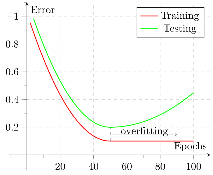
It is usually a good idea to monitor the loss function on the training and validation set as the model is training. Looking at those learning curves is a good indication of overfitting or other problems with model training.

Monitoring the loss function on the training and validation set | *Source*

There are two main options of how this can be done.

Monitor Keras loss using console logs

The quickest and easiest way to log and look at the losses is by simply printing them to the console.

import tensorflow as tf

mnist = tf.keras.datasets.mnist
(x_train, y_train), (x_test, y_test) = mnist.load_data()
x_train, x_test = x_train / 255.0, x_test / 255.0

model = tf.keras.models.Sequential([
   tf.keras.layers.Flatten(input_shape=(28, 28)),
   tf.keras.layers.Dense(512, activation='relu'),
   tf.keras.layers.Dropout(0.2),
   tf.keras.layers.Dense(10, activation='softmax')
])

model.compile(optimizer='sgd',
             loss='sparse_categorical_crossentropy',
             metrics=['accuracy'])

model.fit(x_train, y_train,verbose=1, epochs=10)

Running the code, you can see the loss per epoch is printed directly:

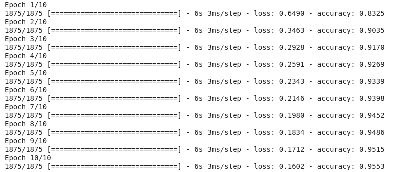
Despite being easy to implement, there are a few issues with this approach:

The logs can be easily lost.
It’s difficult to see progress, especially with higher numbers of epochs.
You might not have access to these logs when working on remote machines.

Using callbacks can be a better alternative.

Monitor Keras losses using a callback

Callbacks are functions passed to other functions, allowing them to be executed after a defined task or event is completed.

We’ll be using neptune.ai as our experiment tracker for the metrics we track with our callback. Neptune is a versatile and highly scalable experiment tracker, allowing you to track months-long training runs and compare thousands of metrics in no time.

Disclaimer

Please note that this article references a deprecated version of Neptune.

For information on the latest version with improved features and functionality, please visit our website.

To get started, make an account (it’s free for personal use!) and check out the Quickstart guide, which includes information on how to connect your Google Colab environment to Neptune. Then, all you’ll have to do is create a project and your API key from the UI.

After that, using callbacks with Neptune is simple. For example, logging your Keras loss to Neptune could look like this:

from keras.callbacks import Callback

class NeptuneCallback(Callback):
    def on_batch_end(self, batch, logs=None):
        for metric_name, metric_value in logs.items():
            neptune_run[f"{metric_name}"].append(metric_value)

    def on_epoch_end(self, epoch, logs=None):
        for metric_name, metric_value in logs.items():
            neptune_run[f"{metric_name}"].append(metric_value)

Here, our callback sends metrics (like loss and accuracy) to Neptune at the end of every batch and epoch so we can visualize them easily.

You can create the monitoring callback yourself or use one of the many available Keras callbacks in the Keras library and other libraries that integrate with it—like neptune.ai, TensorBoard, and others.

Once your callback is ready, you just pass it to model.fit(…). Be sure to specify your API key and the project name before running the code.

import neptune
from neptune.integrations.tensorflow_keras import NeptuneCallback

run = neptune.init_run(
    project='user/keras-loss-tracking',  # Specify your user and project name
    api_token="")  # Specify your API key 
 
neptune_callback = NeptuneCallback(run=run)
 
model.fit(
    x_train,
    y_train,
    validation_split=0.2,
    epochs=10,
    callbacks=[neptune_callback],
)

Now you can easily monitor your experiment learning curves and visualize them like this:

In this dashboard, we’re visualizing many key aspects of our model training: accuracy, loss, hyperparameters, model architecture, and even sample predictions on the test set.

You can interact with this example project directly on the Neptune web app.

Why Keras loss nan happens

Most of the time, losses you log will be just some regular values, but sometimes you might get nans when working with Keras loss functions.

When that happens, your model will not update its weights and will stop learning, so this situation needs to be avoided.

There could be many reasons for nan loss but usually, what happens is:

nans in the training set will lead to nans in the loss,
NumPy infinite in the training set will also lead to nans in the loss,
Using a training set that is not scaled,
Use of very large l2 regularizers and a learning rate above 1,
Use of the wrong optimizer function,
Large (exploding) gradients that result in a large update to network weights during training.

So in order to avoid nans in the loss, ensure that:

Check that your training data is properly scaled and doesn’t contain nans;
Check that you are using the right optimizer and that your learning rate is not too large;
Check whether the l2 regularization is not too large;
If you are facing the exploding gradient problem, you can either: re-design the network or use gradient clipping so that your gradients have a certain “maximum allowed model update”.

Final thoughts

Hopefully, this article gave you some background into loss functions in Keras.

We’ve covered:

Built-in loss functions in Keras,
Implementation of your own custom loss functions,
How to add sample weighing to create observation-sensitive losses,
How to avoid loss nans,
How you can visualize loss as your model is training.

For more information, check out the Keras Repository and the TensorFlow Loss Functions documentation.

Was the article useful?

More about Keras Loss Functions: Everything You Need to Know

Check out our product resources and related articles below:

We are joining OpenAI

Synthetic Data for LLM Training

What are LLM Embeddings: All you Need to Know

Detecting and Fixing ‘Dead Neurons’ in Foundation Models

Explore more content topics:

Computer Vision General LLMOps ML Model Development ML Tools MLOps Natural Language Processing Paper Reflections Reinforcement Learning Tabular Data Time Series

Neptune is the experiment tracker purpose-built for foundation model training.

It lets you monitor and visualize thousands of per-layer metrics—losses, gradients, and activations—at any scale. Drill down into logs and debug training issues fast. Keep your model training stable while reducing wasted GPU cycles.

Play with a live project

See Docs