

Object detection as a task in computer vision
We encounter objects every day in our life. Look around, and you’ll find multiple objects surrounding you. As a human being, you can easily detect and identify each object that you see. It’s natural and doesn’t take much effort.
For computers, however, detecting objects is a task that needs a complex solution. For a computer to “detect objects” means to process an input image (or a single frame from a video) and respond with information about objects on the image and their position. In computer vision terms, we call these two tasks classification and localization. We want the computer to say what kind of objects are presented on a given image and where exactly they’re located.
Multiple solutions have been developed to help computers detect objects. Today, we’re going to explore a state-of-the-art algorithm called YOLO, which achieves high accuracy at real-time speed. In particular, we’ll learn how to train this algorithm on a custom dataset in TensorFlow or Keras.
First, let’s see what exactly YOLO is and what it’s famous for.
YOLO as a real-time object detector
What is YOLO?
YOLO is an acronym for “You Only Look Once” (don’t confuse it with You Only Live Once from The Simpsons). As the name suggests, a single “look” is enough to find all objects on an image and identify them.
In machine learning terms, we can say that all objects are detected via a single algorithm run. It’s done by dividing an image into a grid and predicting bounding boxes and class probabilities for each cell in a grid. In case we’d like to employ YOLO for car detection, here’s what the grid and the predicted bounding boxes might look like:

Source
The image above contains only the final set of boxes obtained after filtering. It’s worth noting that YOLO’s raw output contains many bounding boxes for the same object. These boxes differ in shape and size. As you can see in the image below, some boxes are better at capturing the target object whereas others offered by an algorithm perform poorly.

To select the best bounding box for a given object, a Non-maximum suppression (NMS) algorithm is applied.

All boxes that YOLO predicts have a confidence level associated with them. NMS uses these confidence values to remove the boxes that were predicted with low confidence (that is, below 0.5).
When all uncertain bounding boxes are removed, only the boxes with the high confidence level are left. To select the best one among the top-performing candidates, NMS selects the box with the highest confidence level and calculates how it intersects with the other boxes around. If an intersection is higher than a particular threshold level, the bounding box with lower confidence is removed. In case NMS compares two boxes that have an intersection below a selected threshold, both boxes are kept in the final predictions.
YOLO compared to other detectors
Although a convolutional neural net (CNN) is used under the hood of YOLO, it’s still able to detect objects with real-time performance. It’s possible thanks to YOLO’s ability to do the predictions simultaneously in a single-stage approach.
Other —slower— algorithms for object detection (like Faster R-CNN) typically use a two-stage approach:
- In the first stage, interesting image regions are selected. These are the parts of an image that potentially contain any objects;
- In the second stage, each of these regions is classified using a convolutional neural net.
Usually, there are many regions in an image containing objects. All of these regions are sent to classification. Classification is a time-consuming operation, which is why the two-stage object detection approach performs slower compared to one-stage detection.
YOLO doesn’t select the interesting parts of an image. Instead, it predicts bounding boxes and classes for the whole image in a single forward net pass.
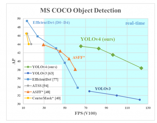
Below you can see how fast YOLO is compared to other popular detectors.

Versions of YOLO
YOLO was first introduced in 2015 by Joseph Redmon in his research paper titled “You Only Look Once: Unified, Real-Time Object Detection”.
Since then, YOLO has evolved a lot. In 2016 Joseph Redmon described the second YOLO version in “YOLO9000: Better, Faster, Stronger”.
About two years after the second YOLO update, Joseph came up with another net upgrade. His paper, called “YOLOv3: An Incremental Improvement”, caught the attention of many computer engineers and became popular in the machine learning community.
In 2020, Joseph Redmon decided to stop researching computer vision, but it didn’t stop YOLO from being developed by others. That same year, a team of three engineers (Alexey Bochkovskiy, Chien-Yao Wang, Hong-Yuan Mark Liao) designed the fourth version of YOLO, even faster and more accurate than before. Their findings are described in the “YOLOv4: Optimal Speed and Accuracy of Object Detection” paper they published on April 23rd, 2020.
Two months after the release of the 4th version, an independent developer, Glenn Jocher, announced the 5th version of YOLO. This time, there was no research paper published. The net became available on Jocher’s GitHub page as a PyTorch implementation. The fifth version had pretty much the same accuracy as the fourth version but it was faster.
Lastly, in July 2020, we got another big YOLO update. In a paper titled “PP-YOLO: An Effective and Efficient Implementation of Object Detector”, Xiang Long and team came up with a new version of YOLO. This iteration of YOLO was based on the 3rd model version and exceeded the performance of YOLO v4.

Using YOLO models in 2025
Since the PP-YOLO paper came out with YOLO v4, the overall YOLO project has improved dramatically, with the latest version being YOLO11. Now, you can find all YOLO versions in a single Python package offered by Ultralytics. It offers fine-tuned YOLO versions for tasks like segmentation, classification, and pose estimation on top of object detection. For the rest of the tutorial, we will use the Ultralytics package as well.
Setting up the environment
Let’s install a few libraries commonly used with ultralytics:
pip install ultralytics opencv-python matplotlib numpy neptune
Here is why we need these libraries:
- OpenCV: transforming and manipulating images before they are fed to YOLO
- Numpy: general matrix manipulation library as images are commonly stored in 3D matrices
- Matplotlib: to plot images
The last library is from neptune.ai. Neptune is an experiment tracking platform designed to simplify and streamline the iterative process of model experimentation. Using Neptune, you can log virtually everything related your experiments such as: model hyperparameters, weights, artifacts, datasets (CSVs, images, video, etc.), or any custom metadata such as plots or metrics to a unified dashboard.
We will use Neptune in the tutorial to log the images we will feed to YOLO, their transformed versions, and custom fine-tuned YOLO models.
Disclaimer
Please note that this article references a deprecated version of Neptune.
For information on the latest version with improved features and functionality, please visit our website.
To get started with Neptune:
- Sign up and create a new project in your dashboard.
- Save your Neptune credentials as environment variables.
How to run pre-trained YOLO out-of-the-box
Now, let’s import the installed libraries and packages:
import os

import cv2
import matplotlib.pyplot as plt
import neptune
from ultralytics import YOLO
We have imported the YOLO class from ultralytics, which will allow us to download model weights directly to our environment in a single line of code.
Before we do anything, let’s write a function to create Neptune run objects:
def init_run(tags=None):
   run = neptune.init_run(
       project="bexgboost/project",
       api_token=os.getenv("NEPTUNE_API_TOKEN"),
       tags=tags,
   )
   return run
Think of run objects as managers of each of your experiments. A single run object creates a single experiment in your Neptune dashboard and all associated metadata will be available inside of it. Notice how the function is using the os library to read the environment variables you stored in the previous section to connect to Neptune.
Object detection with YOLO
Now, let’s load our first YOLO11 model:
MODEL_NAME = "yolo11n.pt"

model = YOLO(MODEL_NAME)

run = init_run(['yolo-detection'])

# Log model configuration
run["model/task"] = model.task
run["model/name"] = MODEL_NAME
In the first line, the n in yolo11n.pt stands for nano. The YOLO11 family of models comes in five sizes:
- n: nano
- s: small
- m: medium
- l: large
- x: extra-large
We are using the nano version as it’s sufficient for our task of processing a few images. However, for larger datasets or more complex tasks, you might consider using the larger versions.
When you pass the model name as a string, it loads as a model object. On the first run, the nano model (5 MB in size) will be downloaded automatically. By default, this model is configured for object detection tasks, which can be confirmed by checking the model’s .task attribute.
We log this task information to our Neptune dashboard using the syntax run[‘model/task’] = model.task, along with the model’s name. This allows us to keep track of the model configuration for each experiment.
Using this model for inference is straightforward and requires only a single line of code:
img1_path = "images/crosswalk.jpg"
img2_path = "images/pedestrians.jpg"
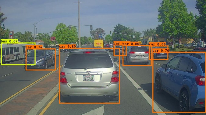
results = model(img1_path)
results is a list containing Result classes:
>>>type(results[0])
ultralytics.engine.results.Results
The results contain information about the detected object names and their bounding box coordinates. To visualize these results, we’ll use the plot() method of the result objects. We’ll then pass the output to the OpenCV library’s cvtColor function for color space conversion. Finally, we’ll display the processed image using Matplotlib’s imshow function. We also upload the output image to Neptune under the predictions/sample namespace:
# Plot and log the results
fig, ax = plt.subplots(figsize=(12, 8))

ax.imshow(cv2.cvtColor(results[0].plot(), cv2.COLOR_BGR2RGB))
ax.axis("off")

# Upload the image to Neptune
run["predictions/sample"].upload(neptune.types.File.as_image(fig))

plt.show()

As you can see, even the 5 MB nano model is capable of correctly identifying the objects in the image.
To end this object detection experiment, call the stop() method of the run object:
run.stop()
Image segmentation with YOLO
We follow a similar syntax for image segmentation. The only difference is that we create a new run object with the yolo-segmentation tag and change the model name to yolo11n-seg.pt to specify that we want the nano segmentation model:
run = init_run(["yolo-segmentation"])

MODEL_NAME = "yolo11n-seg.pt"

model = YOLO(MODEL_NAME)

# Log model configuration
run["model/config"] = model.model.yaml
run["model/task"] = model.task
run["model/name"] = MODEL_NAME
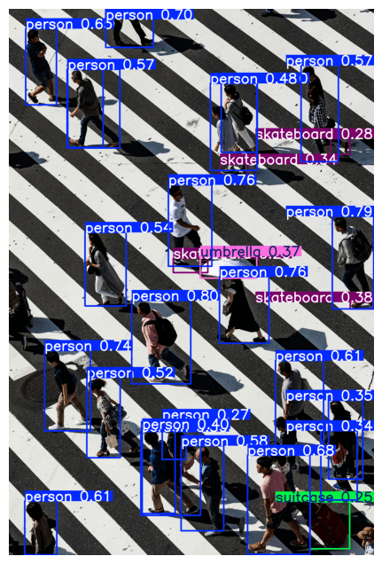
Let’s segment the second image:
results = model(img2_path)

# Plot and log the results
fig, ax = plt.subplots(figsize=(12, 8))
ax.imshow(cv2.cvtColor(results[0].plot(), cv2.COLOR_BGR2RGB))
ax.axis("off")
run["predictions/sample"].upload(neptune.types.File.as_image(fig))
plt.show()

run.stop()

That was a tricky image but the nano model managed to draw accurate segmentation masks for most of the people visible on the crosswalk.
If you want to see how to use YOLO models in Ultralytics for other tasks, refer to the Tasks page of the Ultralytics documentation.
How to fine-tune YOLO on a custom dataset
Ultralytics makes it super easy to fine-tune YOLO models on custom datasets. For example, below we fine-tune the object detector nano model on the COCO128 dataset for five epochs:
run = init_run(["yolo-training"])

MODEL_NAME = "yolo11n.pt"

model = YOLO(MODEL_NAME)

run["model/name"] = MODEL_NAME
run["model/task"] = "training"

# Make sure you run this line with an NVIDIA GPU
results = model.train(data="coco128.yaml", epochs=5, device="0")
Wait for a few minutes for the training to finish and you should see two new folders in your working directory: runs and datasets.
datasets was created when ultralytics downloaded the COCO128 dataset (only happens on first use), while runs was populated as the training took place. We are more interested in the runs directory, so let’s print its contents:
.
└── detect
   └── train
       ├── args.yaml
       ├── labels.jpg
       ├── labels_correlogram.jpg
       ├── results.csv
       ├── train_batch0.jpg
       ├── train_batch1.jpg
       ├── train_batch2.jpg
       ├── val_batch0_labels.jpg
       ├── val_batch0_pred.jpg
       ├── val_batch1_labels.jpg
       ├── val_batch1_pred.jpg
       └── weights
           ├── best.pt
           └── last.pt
Under runs/detect/train/weights, you can see two files: best.pt and last.pt. We are interested in best.pt (pt stands for pre-trained) because it contains the weights for the best model from the training. Let’s use it:
best_model = YOLO("runs/detect/train/weights/best.pt")

results = best_model(img2_path)

# Plot and log the results
fig, ax = plt.subplots(figsize=(12, 8))
ax.imshow(cv2.cvtColor(results[0].plot(), cv2.COLOR_BGR2RGB))
ax.axis("off")
plt.show()
The results are just as good.
Now, let’s log the best model to Neptune:
run["model/fine-tuned"].upload("runs/detect/train/weights/best.pt")

run.stop()
If you want, you can upload other metadata in the runs directory or the dataset itself using the same syntax.
How to find good datasets for fine-tuning YOLO
In the last example, we used the COCO128 dataset, which is part of the larger Common Objects in Context (COCO) project. It provides various COCO datasets for large-scale object detection, segmentation, and captioning tasks, and the COCO128 is only a small version containing 128 images.
If you want more high-quality datasets for fine-tuning YOLO models, refer to the Datasets page of the Ultralytics documentation. It lists more than two dozen high-quality, annotated datasets suitable for fine-tuning Ultralytics YOLO models.
Exploring Neptune dashboard
Now, it is time to visit the Neptune dashboard and explore the metadata you have captured. Here is the dashboard for the community project we have created for this article:


Yours should be similar, containing three experiments with different tags. Let’s open a couple of experiments and look at the metadata:

Conclusions
You’ve just learned how to use YOLO11 for computer vision tasks using the Ultralytics Python package. We have covered object detection, segmentation, and fine-tuning YOLO on a custom dataset. Along the way, you have also learned how to capture experiment artifacts like metadata, model weights, and plots to Neptune.
Curious for more? Check more content on computer vision and AI.
