
Bayesian Neural Networks (BNN) are different from Artificial Neural Networks (NN). The main difference—BNNs can respond “I’m not sure”. Which is interesting, but why would you want a neural network to tell you that it doesn’t know the answer to your question?
To show you why it’s important for a network to say “I’m not sure”, we need to consider dealing with out-of-distribution data. In AI security, the out-of-distribution detection is how the network senses when someone is trying to fool it with examples that don’t come from the dataset.
We’re going to explore the theory behind BNNs, and then implement, train, and run an inference with BNNs for the task of digit recognition. This is tricky, but I’ll show you what you need to do to make BNNs start learning. We’ll code it in the new, hot JAX framework (we’ll do a quick introduction if you don’t know it).
By the end of the article, we will feed our neural network with letters instead of digits and see what it does. Let’s get started!
Bayesian perspective on artificial neural networks

Before we begin, please note that this is a complex topic. If you find the theory hard to understand, go ahead and jump to the coding part of this article. Later, you can also check out additional in-depth guides linked at the end of this article.
In a non-Bayesian artificial neural network model (on the left in the figure above), we train a point estimate of network parameters.
In a Bayesian artificial neural network (on the right in the figure above), instead of a point estimate, we represent our belief about the trained parameters with a distribution. Instead of variables, we have random variables we want to infer from data.
What is the Bayesian Neural Network?
List of Bayesian Neural Network components:
- Dataset D with predictors X (for example, images) and labels Y (for example, classes).
- Likelihood P(D|θ) or P(Y |X, θ) represented with a categorical softmax distribution on logits calculated by a neural network (NN) parameterized with θ, for example, softmax multi-layer perceptron.
- Note: Up to this moment, it’s not different from non-Bayesian NN.
- If we trained it “normally”—with SGD using cross-entropy loss—then we could say that we get a maximum likelihood point estimate of the parameters θ. See “Deep Learning”, Chapter 5.5: Maximum Likelihood Estimation (“Deep Learning. Adaptive Computation and Machine Learning.” MIT Press, 2016)
- However, with Bayesian NN, the parameters come from their distribution. Read further!
- Prior to the neural network parameters, P(θ) is represented with a normal distribution.
- It encodes our prior knowledge (or rather lack of it) of what the parameter values could be.
- However, we suspect these are some small values around zero.
- This assumption comes from our prior knowledge that DNNs tend to work well when we hold their params near 0.
- Posterior P(θ|D) on our NN parameters after seeing the data—one could say “after the training”.
- Here it is—the distribution of trained parameters.
- We will calculate it using Bayes’ Theorem…
- …or at least we’ll try to do so.
Bayes’ theorem
Bayes’ Theorem, in theory, is the tool we should use to calculate the posterior on NN parameters, based on the prior and the likelihood. But, there’s a catch.

This integral is intractable to calculate. It’s only tractable in a few special cases requiring the use of conjugate priors. Read more about it in “Deep Learning”, Chapter 5.6: Bayesian Statistics (“Deep Learning. Adaptive Computation and Machine Learning.” MIT Press, 2016). There’s also a great article about conjugate priors at Towards Data Science.
In our case, it’s intractable because there’s no analytical solution to this integral. We use a complicated, non-linear function named “artificial neural network”. It’s also computationally intractable because there’s an exponential number of possible parameter assignments to evaluate and sum over in the denominator.
Imagine a binary NN which has 2N parameter assignments for N parameters. For N=272, it’s 2272, which is already more than the amount of atoms in the visible universe. And let’s agree, the 272 parameters aren’t that much, knowing that modern CNN-s have millions of parameters.
Variational Inference to the rescue!
Can’t calculate? Then approximate!

We’ll approximate the posterior with a distribution Q, called a variational distribution, minimizing the KL divergence between them DKL(Q(θ) || P(θ|D)). We’ll find the closest probability distribution to the posterior that is represented by a small set of parameters—like means and variances of a multivariate Gaussian distribution—and we know how to sample from it.
Moreover, we have to be able to backpropagate through it and modify parameters of the distribution (i.e. mean and variance) a little bit each time to see if the resulting distribution is closer to the posterior that we want to calculate.
How do we know if the resulting distribution is closer to the posterior if the posterior is exactly what we want to calculate? That’s the idea!
From the KL divergence between the distributions, DKL(Q(θ) || P(θ|D)), we can get to the Evidence Lower Bound (ELBO).
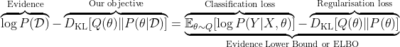
This is called variational inference. It changes the inference problem into an optimization problem. By optimizing the right-hand side, we optimize the classic maximum likelihood classification loss (e.g. the cross-entropy loss) on sampled from our variational distribution NN parameters, θ ∼ Q(·), minus the regularisation loss—which for the Gaussian distribution takes the closed-form, meaning it’s the well-known equation you will see in a minute.
By optimizing it, we maximize the evidence—probability of our dataset being true—and minimize the divergence between our variational distribution, Q(θ), and the posterior, P(θ|D). The posterior is exactly what we wanted, it’s our objective!
One more note: it’s called Evidence Lower Bound because the KL divergence will always be positive. Hence, the right-hand side is the lower bound on the evidence on the left-hand side. See this tutorial for details: Doersch, Carl. ‘Tutorial on Variational Autoencoders’.
Now, as promised, we have the distribution on the NN parameters, Q(θ), and we know how to learn it using ELBO. Let’s jump into the code to see it in practice!
What is JAX?
As I mentioned before, we’ll be using JAX.
“JAX is Autograd and XLA, brought together for high-performance numerical computing and machine learning research. It provides composable transformations of Python+NumPy programs: differentiate, vectorize, parallelize, Just-In-Time compile to GPU/TPU, and more.” ~ JAX documentation.
You can check out the JAX documentation, but you probably don’t need it to understand the code below. As the authors said, it’s like NumPy for machine learning and deep learning research. But, I recommend at least one section to read, the section on Random Numbers. It might be unintuitive because normally you don’t have to think about the state of the pseudo-random number generator in NumPy, but in JAX you pass it explicitly to the function that samples random values.
Bayesian Neural Networks for digits classification using JAX
You can find the code here. README tells you how to run it. I encourage you to do it now and then finish reading this article. This repo includes:
- mlp.py – MLP classifier on MNIST (in JAX and Haiku).
- vae.py – Bernoulli VAE generative model on MNIST.
- bayes.py – Variational Bayes NN classifier on MNIST.
Today, we’ll do the last one, the Variational Bayesian NN classifier. We’ll go through the most important points in the code.
Note on HumbleSL (the hsl package)
HumbleSL is straightforward supervised learning (SL) Python library that I wrote. It provides all the boilerplate code needed to do Deep SL:
- a network definition factory,
- metrics and losses,
- a data loader,
- train loop,
- etc.
It’s backed by the JAX library and the Haiku framework. It uses TensorFlow Datasets for data loading and preprocessing.
Training
Download MNIST dataset
Lines 56-61 download training and test datasets.
train_dataset = hsl.load_dataset(
     'mnist:3.*.*', 'train', is_training=True, batch_size=FLAGS.batch_size)
 train_eval_dataset = hsl.load_dataset(
     'mnist:3.*.*', 'train', is_training=False, batch_size=10000)
 test_eval_dataset = hsl.load_dataset(
     'mnist:3.*.*', 'test', is_training=False, batch_size=10000)
train_dataset is used for training. train_eval_dataset is used for performance evaluation on the training dataset. test_eval_dataset is used for, you guessed it, performance evaluation on the test dataset.
The datasets are iterators, you access the consecutive batches of images (and labels) this way:
batch_image, batch_label = next(train_dataset)
Create multi-layer perceptron (MLP) model
Lines 71-74 create the MLP model.
net = hk.without_apply_rng(hk.transform(
     hsl.mlp_fn,
     apply_rng=True  # In the process of being removed. Can only be `True`.
 ))
If you’re interested in what exactly this snippet does, please check the Haiku Fundamentals. All you need to know is that it creates the “standard” MLP with two hidden layers of 64 units.
It takes a 28×28 image on the input and returns 10 values corresponding to each possible class (digit). The net object has two functions: init, and apply.
- params = net.init(next(rng), batch_image) takes the next random generator state and the batch of images, and returns the initial model parameters. It needs the random generator state to sample the parameters.
- logits = net.apply(params, batch_image) takes the model parameters and the batch of images, then returns the batch output (batch of 10 numbers).
You can think of the net as the model bare architecture. You need to provide it with some parameters in order to predict it.
Initialize Bayesian NN parameters
Lines 79-85 take the MLP model parameters and use it to initialize the Bayesian NN parameters.
prior = dict(
     # Haiku inits weights to trun. normal, with stddev ``1 / sqrt(fan_in)``.
     # Where ``fan_in`` is the number of incoming connection to the layer.
     mu=params,
     # Init to ~0.001 variance around default Haiku initialization.
     logvar=jax.tree_map(lambda x: -7 * jnp.ones_like(x), params),
 )
We use the mean-field approximation to the posterior. It means that we represent our variational distribution with the Gaussian distribution parametrized with mean and variance — or log-variance, as it can take any values, not only positive, which simplifies the training. We do it because it’s easy to sample from the Gaussian distribution.
Remember here, the posterior is the distribution of trained MLP parameters. We don’t have one set of MLP parameters to train. We train the variational distribution that approximates the posterior and sample the MLP parameters from it. In code, for variables name, I might use aprx_posterior, posterior, and prior interchangeably to represent the variational distribution, which I admit isn’t 100% correct, but in practice, they are the same thing or I wanted to stress out stage of trained parameters (i.e. prior is untrained posterior).
Initialize optimizer
Lines 89-90 define and initialize the ADAM optimizer.
opt = optix.adam(FLAGS.lr)
 opt_state = opt.init(prior)
It is as simple as that. You pass the learning rate, FLAGS.lr, and the initial parameters, prior. Of course, the optimizer is used to apply the gradients onto the parameters. The same as in the standard deep learning.
Define objective
Lines 92-110 define the ELBO objective.
def elbo(aprx_posterior, batch, rng):
     """Computes the Evidence Lower Bound."""
     batch_image, batch_label = batch
     # Sample net parameters from the approximate posterior.
     params = sample_params(aprx_posterior, rng)
     # Get network predictions.
     logits = net.apply(params, batch_image)
     # Compute log likelihood of batch.
     log_likelihood = -hsl.softmax_cross_entropy_with_logits(
         logits, batch_label)
     # Compute the kl penalty on the approximate posterior.
     kl_divergence = jax.tree_util.tree_reduce(
         lambda a, b: a + b,
         jax.tree_multimap(hsl.gaussian_kl,
                           aprx_posterior['mu'],
                           aprx_posterior['logvar']),
    )
     elbo_ = log_likelihood - FLAGS.beta * kl_divergence
     return elbo_, log_likelihood, kl_divergence
It takes the batch of images (and labels), samples the MLP parameters, and runs prediction on them. Then, it calculates the cross-entropy between the logits and the labels (classification loss) and computes the KL divergence between the variational distribution and the normal distribution (regularization loss).
hsl.gaussian_kl calculates the latter in the closed-form. Combination of the two, weighted by FLAGS.beta, yields ELBO. This matches the mathematical expression for ELBO above. Loss is the negative ELBO:
def loss(params, batch, rng):
     """Computes the Evidence Lower Bound loss."""
     return -elbo(params, batch, rng)[0]
We need to take the negation because JAX optimizers can only do the gradient descent. However, we need to maximize ELBO, not minimize it.
Training loop
Lines 116-126 define the SGD update step. This is the final piece we need to run the training.
@jax.jit
 def sgd_update(params, opt_state, batch, rng):
     """Learning rule (stochastic gradient descent)."""
     # Use jax transformation `grad` to compute gradients;
     # it expects the prameters of the model and the input batch
     grads = jax.grad(loss)(params, batch, rng)
     # Compute parameters updates based on gradients and optimiser state
     updates, opt_state = opt.update(grads, opt_state)
     # Apply updates to parameters
     posterior = optix.apply_updates(params, updates)
     return posterior, opt_state
This function does one step of the SGD update. Firstly, it evaluates the gradient of the loss function for the current parameters and the batch of data. Then, the update is computed and applied to the parameters. This function returns the new variational distribution parameters and the optimizer state after one update. The latter is needed because the ADAM optimizer stores and updates the state required by its adaptive moment estimation.
Now, you simply run this function in the loop and the training will progress. I have the helper function for this: hsl.loop. It also takes care of checkpointing and periodic evaluation of the train and test performance.
Evaluation
Lines 128-140 calculate diagnostics.
def calculate_metrics(params, data):
     """Calculates metrics."""
     images, labels = data
     probs = predict(net, params, images, next(rng), FLAGS.num_samples)[0]
     elbo_, log_likelihood, kl_divergence = elbo(params, data, next(rng))
     mean_aprx_evidence = jnp.exp(elbo_ / FLAGS.num_classes)
     return {
         'accuracy': hsl.accuracy(probs, labels),
         'elbo': elbo_,
         'log_likelihood': log_likelihood,
         'kl_divergence': kl_divergence,
         'mean_approximate_evidence': mean_aprx_evidence,
    }
It starts with running the prediction on the provided parameters and data. It’s different from simply sampling one set of parameters as in the ELBO objective. The next subsection describes it. These predictions are used together with ground truth labels to calculate the accuracy—the hsl.accuracy helper function.
Next, we calculate ELBO, the classification loss (log_likelihood), and the regularisation loss (kl_divergence). ELBO is used to calculate the approximate evidence, which follows directly from the formula for ELBO—it’s evidence lower-bound, isn’t it? It is the approximate probability of the data—that images have the corresponding labels—under the current parameters. The higher the better, because it means that our model fits the data well—it gives a high probability to the labels from the dataset.
All of these metrics are put together into a dictionary and returned to the caller. In our case, the hsl.loop helper function will call it from time to time on the data from the train and test datasets and the current parameters.
Prediction
Lines 41-49 run prediction.
def predict(net, prior, batch_image, rng, num_samples):
     probs = []
     for i in range(num_samples):
         params_rng, rng = jax.random.split(rng)
         params = sample_params(prior, params_rng)
         logits = net.apply(params, batch_image)
         probs.append(jax.nn.softmax(logits))
     stack_probs = jnp.stack(probs)
     return jnp.mean(stack_probs, axis=0), jnp.std(stack_probs, axis=0)
This simply runs prediction on sample num_samples sets of parameters. Then, the predictions are averaged, and the standard deviation of these predictions is calculated as the measure of uncertainty.
Speaking about uncertainty, now that we have all the parts, let’s play with this Bayesian NN a little.
Playing with Bayesian Neural Networks
You run the code and see this:
      0 | test/accuracy                       0.122
      0 | test/elbo                         -94.269
      0 | test/kl_divergence                 26.404
      0 | test/log_likelihood               -67.865
      0 | test/mean_approximate_evidence     0.000
      0 | train/accuracy                     0.095
      0 | train/elbo                       -176.826
      0 | train/kl_divergence               26.404
      0 | train/log_likelihood             -150.422
      0 | train/mean_approximate_evidence     0.000
These are diagnostics before the training and they seem okay:
- Accuracy is ~10%, which is perfectly fine for randomly initialized NN. This is accuracy for guessing labels at random.
- ELBO is very low, which is okay at the beginning, as our variational distribution is far away from the true posterior.
- KL divergence between the variational distribution and the normal distribution is positive. It must be positive because we calculated it in closed-form and KL, because it’s a measure of distance, can’t take negative values.
- Log-likelihood, or log probabilities of the true labels returned by the MLP model, is very low. This means that the model assigns low probabilities to the true labels. It’s expected if we didn’t train it yet.
- The mean approximate evidence is 0. Again, we didn’t train the model yet, so it doesn’t model the dataset at all.
Let’s run it for 10k steps and see the diagnostics again:
  10000 | test/accuracy                       0.104
  10000 | test/elbo                         -5.796
  10000 | test/kl_divergence                 2.516
  10000 | test/log_likelihood               -3.280
  10000 | test/mean_approximate_evidence     0.560
  10000 | train/accuracy                     0.093
  10000 | train/elbo                         -5.610
  10000 | train/kl_divergence                 2.516
  10000 | train/log_likelihood               -3.095
  10000 | train/mean_approximate_evidence     0.571
It isn’t good. The probabilities of the true labels went up, log_likelihood and
mean_approximate_evidence went up, the variational distribution got closer to the normal distribution, kl_divergence got lower.
However, the accuracy, which takes argmax of the returned probabilities to infer the label and compare it with the ground truth label, is still ~10% as good as the random classifier. This isn’t a bug in the code. The diagnostics are correct and we need two tricks to make it train. Keep reading!
Tricks to make Bayesian Neural Networks train
Low beta
The beta parameter weights the classification loss and the regularization loss. The higher the beta, the stronger the regularization. Too strong regularization will constrain the model too much and it won’t be able to encode any knowledge. In the example above, it was set to FLAGS.beta = 1.
This caused kl_divergance (regularization loss) to go down considerably. However, it’s too strong! The better value is around FLAGS.beta = 0.001 and this is the default value in the code I provided you with.
Low initial variance
Another thing is the initial variance of the variational distribution. Too big and again, the network has a hard time starting training and encoding any useful knowledge in it. It is because the sampled parameters vary a lot. In the example above it was set to ~0.37. In the code, by default, it’s set to ~0.001 and it’s a much better value.
Fixed example
Now that we changed the hyperparameters to the correct one, let’s see the diagnostics after 10k steps:
  10000 | test/accuracy                       0.979
  10000 | test/elbo                         -0.421
  10000 | test/kl_divergence               318.357
  10000 | test/log_likelihood               -0.103
  10000 | test/mean_approximate_evidence     0.959
  10000 | train/accuracy                     0.995
  10000 | train/elbo                         -0.341
  10000 | train/kl_divergence               318.357
  10000 | train/log_likelihood               -0.022
  10000 | train/mean_approximate_evidence     0.966
With the test accuracy of 98%, we can agree it works now! Note how big is the regularization loss (kl_divergence).
Yes, it’s that far from the normal distribution, but it needs to be. Nonetheless, with this little beta, it still prevents overfitting. Mean approximate evidence is also very high, which means that our model predicts the data well. Note that ELBO is quite close to zero too (which is its maximum value).
Finding out-of-distribution examples

I took the trained model and ran it on the digit “3” and the letter “B” above. Here’s the output:
|
|
Prediction
|
Probability
|
Std. dev. (uncertainty)
|
|
Digit “3” |
3 |
100% |
0
|
|
Letter “B” |
8 |
57% |
0,45 |
As you can see, it doesn’t have any problem classifying the digit “3” as three. However, an interesting thing happens when we feed it with something it didn’t see during training. The model classifies the letter “B” as eight. If we were dealing with a normal neural network, that would be it.
Luckily, the Bayesian neural network we’ve trained can also tell us how certain it is.
We see that in the case of the digit “3”, it’s confident—std. dev. around the probability is 0. For the letter “B”, it returns that the probability can vary as much as 0,45 in either direction!
This is like our model telling us “if I had to guess, then this is 8, but it could be anything—I haven’t seen this before.”
This way the Bayesian NN can either classify the image or say “I don’t know”. We could figure out the std. dev. threshold after which we reject the classification from, for example, the test dataset we evaluated our model with.
I simply run the model on the whole test dataset and observe the std. dev. values of its predictions. Then, I take the 99th percentile (the value for which 99% of other values are lower), which in this case is 0,37. So, I decide that the classifications for the 1% of the test images should be rejected.
I do this because I know there are some crazy images in the MNIST dataset that even I can’t classify correctly. Coming back to our example, clearly 0,45 > 0,37, so we should reject the classification for the letter “B”.
Conclusion
That’s it! Now you can train a neural network that won’t allow you to fool it. Uncertainty estimation is a big theme in AI safety. I leave you with the further reading list:
- A great post on Bayesian Inference — Intuition and Example.
- Learn about conjugate prior and why it’s important, read here.
- Derive and understand ELBO, read here.
- A Beginner’s Guide to Variational Methods: Mean-Field Approximation.
- The problem of approximate inference in Variational Inference: A Review for Statisticians.
- Making Your Neural Network Say “I Don’t Know” — Bayesian NNs using Pyro
