Exploring Clustering Algorithms: Explanation and Use Cases

Clustering (cluster analysis) is grouping objects based on similarities. Clustering can be used in many areas, including machine learning, computer graphics, pattern recognition, image analysis, information retrieval, bioinformatics, and data compression.

Clusters are a tricky concept, which is why there are so many different clustering algorithms. Different cluster models are employed, and for each of these cluster models, different algorithms can be given. Clusters found by one clustering algorithm will definitely be different from clusters found by a different algorithm.

In machine learning systems, we often group examples as the first step towards understanding the dataset. Grouping an unlabelled example is called clustering. As the samples are unlabelled, clustering relies on unsupervised machine learning. If the examples are labeled, then it becomes classification.

Knowledge of cluster models is fundamental if you want to understand the differences between various cluster algorithms, and in this article, we’re going to explore this topic in depth.

What are clustering algorithms?

Clustering algorithms are used to group data points based on certain similarities. There’s no criterion for good clustering. Clustering determines the grouping with unlabelled data. It mainly depends on the specific user and the scenario.

Typical cluster models include:

• Connectivity models – like hierarchical clustering, which builds models based on distance connectivity.
• Centroid models – like K-Means clustering, which represents each cluster with a single mean vector.
• Distribution models – here, clusters are modeled using statistical distributions.
• Density models – like DBSCAN and OPTICS, which define clustering as a connected dense region in data space.
• Group models – these models don’t provide refined results. They only offer grouping information.
• Graph-based models – a subset of nodes in the graph such that an edge connects every two nodes in the subset can be considered as a prototypical form of cluster.
• Neural models – self-organizing maps are one of the most commonly known Unsupervised Neural networks (NN), and they’re characterized as similar to one or more models above.

Note, there are different types of clustering:

• Hard clustering – the data point either entirely belongs to the cluster, or doesn’t. For example, consider customer segmentation with four groups. Each customer can belong to either one of four groups.
• Soft clustering – a probability score is assigned to data points to be in those clusters.

In this article, we’ll focus on the first four (connectivity, centroid, distribution, and density models).

Types of clustering algorithms and how to select one for your use case

Let’s look at types of clustering algorithms and how to choose them for your use case.

Hierarchical clustering algorithms (connectivity-based clustering)

The main idea of hierarchical clustering is based on the concept that nearby objects are more related than objects that are farther away. Let’s take a closer look at various aspects of these algorithms:

• The algorithms connect to “objects” to form “clusters” based on their distance.
• A cluster can be defined by the max distance needed to connect to the parts of the cluster.
• Dendrograms can represent different clusters formed at different distances, explaining where the name “hierarchical clustering” comes from. These algorithms provide a hierarchy of clusters that at certain distances are merged.
• In the dendrogram, the y-axis marks the distance at which clusters merge. The objects are placed beside the x-axis such that clusters don’t mix.

Hierarchical clustering is a family of methods that compute distance in different ways. Popular choices are known as single-linkage clustering, complete linkage clustering, and UPGMA. Furthermore, hierarchical clustering can be:

1. Agglomerative – it starts with an individual element and then groups them into single clusters.
2. Divisive – it starts with a complete dataset and divides it into partitions.

Agglomerative hierarchical clustering (AHC)

In this section, I’ll be explaining the AHC algorithm which is one of the most important hierarchical clustering techniques. The steps to do it are:

1. Each data point is treated as a single cluster. We have K clusters in the beginning. At the start, the number of data points will also be K.
2. Now we need to form a big cluster by joining 2 closest data points in this step. This will lead to total K-1 clusters.
3. Two closest clusters need to be joined now to form more clusters. This will result in K-2 clusters in total. 
4. Repeat the above three steps until K becomes 0 to form one big cluster. No more data points are left to join.
5. After forming one big cluster at last, we can use dendrograms to split the clusters into multiple clusters depending on the use case.

The image below gives an idea of the hierarchical clustering approach.

Advantages of AHC:

• AHC is easy to implement, it can also provide object ordering, which can be informative for the display.
• We don’t have to pre-specify the number of clusters. It’s easy to decide the number of clusters by cutting the dendrogram at the specific level.
• In the AHC approach smaller clusters will be created, which may uncover similarities in data.

Disadvantages of AHC:

• The objects which are grouped wrongly in any steps in the beginning can’t be undone.

• Hierarchical clustering algorithms don’t provide unique partitioning of the dataset, but they give a hierarchy from which clusters can be chosen. 
• They don’t handle outliers well. Whenever outliers are found, they will end up as a new cluster, or sometimes result in merging with other clusters.

The Agglomerative Hierarchical Cluster Algorithm is a form of bottom-up clustering, where each data point is assigned to a cluster. Those clusters then get connected together. Similar clusters are merged at each iteration until all the data points are part of one big root cluster.

Clustering dataset

Getting started with clustering in Python through Scikit-learn is simple. Once the library is installed, a variety of clustering algorithms can be chosen.

We will be using the `make_classification` function to generate a data set from the `sklearn` library to demonstrate the use of different clustering algorithms. The `make_classification` function accepts the following arguments:

• The number of samples.
• A total number of features.
• The number of informative features.
• The number of redundant features.
• The number of duplicate features drawn randomly from redundant and informative features.
• The number of clusters per class.

from numpy import where
from numpy import unique
from sklearn.datasets import make_classification
from sklearn.cluster import AgglomerativeClustering
import matplotlib.pyplot as plot

# Initializing data
train_data, _ = make_classification(n_samples=1000,
                                       n_features=2,
                                       n_informative=2,
                                       n_redundant=0,
                                       n_clusters_per_class=1,
                                       random_state=4)

agg_mdl = AgglomerativeClustering(n_clusters=4)

# each data point assigned to cluster
agg_result = agg_mdl.fit_predict(train_data)

# Obtain all clusters which are unique
agg_clusters = unique(agg_result)

# plot clusters
for agg_cluster in agg_clusters:
    # fetch data point that fall in this clstr
    index = where(agg_result == agg_cluster)

    plot.scatter(train_data[index, 0], train_data[index,1])

# Agglomerative hierarchy plot
plot.show()

Hierarchical clustering is often used in the form of descriptive modeling rather than predictive. It doesn’t work well on large datasets, it provides the best results in some cases only. Sometimes it’s also difficult to detect the correct number of clusters from a dendogram.

Centroid-based clustering algorithms / Partitioning clustering algorithms

In centroid/partitioning clustering, clusters are represented by a central vector, which may not necessarily be a member of the dataset. Even in this particular clustering type, the value of K needs to be chosen. This is an optimization problem: finding the number of centroids or the value of K and assigning the objects to nearby cluster centers. These steps need to be performed in such a way that the squared distance from clusters is maximized.

One of the most widely used centroid-based clustering algorithms is K-Means, and one of its drawbacks is that you need to choose a K value in advance.

K-Means clustering algorithm

The K-Means algorithm splits the given dataset into a predefined(K) number of clusters using a particular distance metric. The center of each cluster/group is called the centroid.

How does the K-Means algorithm work?

Let’s see how the K-Means algorithm works:

• Initially, a K number of centroids is chosen. There are different methods for selecting the right value for K.
• Shuffle the data and initialize centroids—randomly select K data points for centroids without replacement.
• Create new centroids by calculating the mean value of all the samples assigned to each previous centroid.
• Randomly initialize the centroid until there’s no change in the centroid, so the assignment of data points to the cluster isn’t changing.
• K-Means clustering uses the Euclidean Distance to find out the distance between points.

Note: An example of K-Means clustering is explained with customer segmentation examples in the use cases section below.

There are two methods to choose the correct value of K: Elbow and Silhouette.

The Elbow method

The Elbow method picks the range of values and takes the best among them. It calculates the Within Cluster Sum of Square(WCSS) for different values of K. It calculates the sum of squared points and calculates the average distance.

In the above formula, Yi is the centroid for the observation of Xi. The value of K needs to be chosen where WCSS starts to diminish. In the plot WCSS versus K, this shows up as an elbow.

The Silhouette method

The Silhouette score/coefficient(SC) is calculated using average intra-cluster distance(m) and an average of the nearest cluster distance(n) for each sample.

In the above formula, n is the distance between a data point and the nearest cluster that the data point is not part of. We can calculate the average SC on all the samples and use this as a metric to decide the number of clusters. 

The SC value ranges between -1 to 1. 1 means clusters are separated well and are distinguishable. The Clusters are wrongly assigned if the value is -1.

These are some of the advantages K-Means poses over other algorithms:

• It’s straightforward to implement.
• It’s scalable to massive datasets and also faster for large datasets.
• It adapts to new examples very frequently.

K-Medians is another clustering algorithm relative to the K-Means algorithm, except cluster centers are recomputed using the median. Sensitivity towards outliers is less in the K-Median algorithm since sorting is required to calculate the median vector slower for large datasets.

K-Means has some disadvantages; the algorithm may provide different clustering results on different runs as K-Means begins with random initialization of cluster centers. The chances are that the results obtained might not be repeated.

Other drawbacks posed by the K-Means algorithm are:

• K-Means clustering is good at capturing the structure of the data if the clusters have a spherical-like shape. It always tries to construct a nice spherical shape around the centroid. This means that the minute the clusters have different geometric shapes, K-Means does a poor job clustering the data.
• Even when the data points belong to the same cluster, K-Means doesn’t allow the data points far from one another, and they share the same cluster.
• K-Means algorithm is sensitive to outliers.
• As the number of dimensions increases, scalability decreases.

Here are some points to remember when using K-Means for clustering:

• Standardize the data when applying the K-Means algorithm, because it will help you get good quality clusters and improve the performance of the clustering algorithm. Since K-Means use a distance-based measure to find the similarity between data points, it’s good to standardize the data to have a standard deviation of one and a mean of zero. Usually, the features present in any dataset would have different units of measurement, for example, income versus age.
• K-Means give more weight to bigger clusters.
• The elbow method used to select the number of clusters doesn’t work well as the error function decreases for all Ks.
• If there’s overlap between clusters, K-Means doesn’t have an intrinsic measure for uncertainty for the examples belonging to the overlapping region to determine which cluster to assign each data point.
• K-Means clusters data even if it can’t be clustered, such as data that comes from uniform distributions.

Mini-Batch K-Means clustering algorithm

K-Means is one of the popular clustering algorithms, mainly because of its good time performance. When the size of the data set increases, K-Means will result in a memory issue since it needs the entire dataset. For those reasons, to reduce the time and space complexity of the algorithm, an approach called Mini-Batch K-Means was proposed.

The Mini-Batch K-Means algorithm tries to fit the data in the main memory in a way where the algorithm uses small batches of data that are of fixed size chosen at random. Here are a couple of points to note about the Mini-Batch K-Means algorithm:

• Clusters are updated (depending on the previous location of cluster centroids) in each iteration by obtaining new arbitrary samples from the dataset, and these steps are repeated until convergence.
• Some of the research suggests that this method saves significant computational time with a trade-off, a little bit of loss in cluster quality. But intense research hasn’t been done to quantify the number of clusters or their size that will impact the cluster quality.

• The location of the clusters is updated based on the new points from each batch.
• The update made is the gradient descent update, which is notably faster than normal batch K-Means.

Density-based clustering algorithms

Density-based clustering connects areas of high example density into clusters. This allows for arbitrary shape distributions as long as dense regions are connected. With the higher dimension data and data of varying densities, these algorithms run into issues. By design, these algorithms don’t assign outliers to clusters.

DBSCAN

The most popular density-based method is Density-Based Spatial Clustering of Applications with Noise (DBSCAN). It features a well-defined cluster model called “density reachability”. 

This type of clustering technique connects data points that satisfy particular density criteria (minimum number of objects within a radius). After DBSCAN clustering is complete, there are three types of points: core, border, and noise.

If you look at the above figure, the core is a point that has some (m) points within a particular (n) distance from itself. The border is a point that has at least one core point at distance n. 

Noise is a point that is neither border nor core. Data points in sparse areas required to separate clusters are considered noise and broader points.

DBSCAN uses two parameters to determine how clusters are defined:

• minPts: for a region to be considered dense, the minimum number of points required is `minPts`.
• eps: to locate data points in the neighborhood of any points, `eps (ε)` is used as a distance measure.

Here’s a step-by-step explanation of the DBSCAN algorithm:

• DBSCAN starts with a random data point (non-visited points).
• The neighborhood of this point is extracted using a distance epsilon ε.
• The clustering procedure starts if there are sufficient data points within this area and the current data point becomes the first point in the newest cluster, or else the point is marked as noise and visited.
• The point within its epsilon ε distance neighborhood also becomes a part of the same cluster for the first point in the new cluster. For all the new data points added to the cluster above, the procedure for making all the data points belong to the same cluster is repeated.
• The above two steps are repeated until all points in the cluster are determined. All points within the ε neighborhood of the cluster have been visited and labeled. Once we’re done with the current cluster, a new unvisited point is retrieved and processed, leading to further discovery of the cluster or noise. The procedure is repeated until all the data points are marked as visited.

An exciting property of DBSCAN is its low complexity. It requires a linear number of range queries on the database. 

The main problem with DBSCAN is:

• It expects some kind of density drop to detect cluster borders. DBSCAN connects areas of high example density. The algorithm is better than K-Means when it comes to oddly shaped data.

One great thing about the DBSCAN algorithm is:

• It doesn’t require a predefined number of clusters. It also identifies noise and outliers. Furthermore, arbitrarily sized and shaped clusters are found pretty well by the algorithm.

from numpy import where
from numpy import unique
from sklearn.datasets import make_classification
from sklearn.cluster import DBSCAN
import matplotlib.pyplot as plot

# Initialize  data
train_data, _ = make_classification(n_samples=1000,
                                       n_features=2,
                                       n_informative=2,
                                       n_redundant=0,
                                       n_clusters_per_class=1,
                                       random_state=4)

# Define model
dbscan_model = DBSCAN(eps=0.25, min_samples=9)

# Train the model
dbscan_model.fit(train_data)

# Assign each data point to a cluster
dbscan_res = dbscan_model.fit_predict(train_data)

# obtain all the unique clusters
dbscan_clstrs = unique(dbscan_res)

# Plot the DBSCAN clusters
for dbscan_clstr in dbscan_clstrs:
    # Obtain data point that belong in this cluster
    index = where(dbscan_res == dbscan_clstr)
    # plot
    plot.scatter(train_data[index, 0], train_data[index, 1])

# show plot
plot.show()

Distribution-based clustering algorithms

The clustering model that’s closely related to statistics is based on distribution models. Clusters can then be defined as objects that belong to the same distribution. This approach closely resembles how artificial datasets are generated, by sampling random objects from distribution. 

While the theoretical aspects of these methods are pretty good, these models suffer from overfitting.

Gaussian mixture model

Gaussian mixture model (GMM) is one of the types of distribution-based clustering. These clustering approaches assume data is composed of distributions, such as Gaussian distributions. In the figure below, the distribution-based algorithm clusters data into three Gaussian distributions. As the distance from the distribution increases, the probability that the point belongs to the distribution decreases. 

GMM can be used to find clusters in the same way as K-Means. The probability that a point belongs to the distribution’s center decreases as the distance from the distribution center increases. The bands show a decrease in probability in the below image. Since GMM contains a probabilistic model under the hood, we can also find the probabilistic cluster assignment. When you don’t know the type of distribution in data, you should use a different algorithm.

Let’s see how GMM calculates probabilities and assigns it to data point:

• A GM is a function composed of several Gaussians, each identified by k ∈ {1,…, K}, where K is the number of clusters. Each Gaussian K in the mixture is comprised of following parameters:
  • A mean μ that defines its center.
  • A covariance Σ that defines its width.
  • A mixing probability that defines how big or small or big the Gaussian function will be.

These parameters can be seen in the below image:

To find the covariance, mean, variance and weights of clusters, GMM uses the Expectation Maximization technique.

Consider we need to assign K number of clusters, meaning K Gaussian distributions, with the mean and covariance values to be μ1, μ2, .. μk and Σ1, Σ2, .. Σk. There’s another parameter Πi which represents the density of distribution. 

To define the Gaussian distribution we need to find the values for these parameters. We’ve already decided on the number of clusters and have assigned the value for mean, covariance, and density. Next are the Expectation step and Maximizations step, which you can check out in this post.

Advantages of GMM

• One of the advantages of GMM over K-Means is that K-Means doesn’t account for variance (here, variance refers to the width of the bell-shaped curve) and GMM returns the probability that data points belong to each of K clusters. 
• In case of overlapped clusters, all the above clustering algorithms fail to identify it as one cluster. 
• GMM uses a probabilistic approach and provides probability for each data point that belongs to the clusters. 

Disadvantages of GMM

• Mixture models are computationally expensive if the number of distributions is large or the dataset contains less observed data points.
• It needs large datasets and it’s hard to estimate the number of clusters.

Let’s now look at how GMM clusters data. The code below helps you to:

• create the data,
• fit the data to the `GaussianMixture` model,
• find the data points that are assigned to a cluster,
• obtain the unique clusters, and
• plot the clusters as shown below.

from numpy import where
from numpy import unique
from sklearn.datasets import make_classification
from sklearn.mixture import GaussianMixture
import matplotlib.pyplot as plot

#init data
train_data, _ = make_classification(n_samples=1200,
                                       n_features=3,
                                       n_informative=2,
                                       n_redundant=0,
                                       n_clusters_per_class=1,
                                       random_state=4)

gaussian_mdl = GaussianMixture(n_components=3)

# model training
gaussian_mdl.fit(train_data)

# data points assigned to a cluster
gaussian_res = gaussian_mdl.fit_predict(train_data)

# get clusters which are unique
gaussian_clstr = unique(dbscan_res)

# Plot 
for gaussian_cluser in gaussian_clstr:

    index = where(gaussian_res == gaussian_cluser)
    # plot
    plot.scatter(train_data[index, 0], train_data[index, 1])

# show plot
plot.show()

Applications of clustering in different fields

Some of the domains in which clustering can be applied are:

• Marketing: customer segment discovery.
• Library: to cluster different books based on topics and information.
• Biology: classification among different species of plants and animals.
• City planning: analyze the value of houses based on location.
• Document Analysis: various research data and documents can be grouped according to certain similarities. Labeling large data is really difficult. Clustering can be helpful in these cases to cluster text & group it into various categories. Unsupervised techniques like LDA are also beneficial in these cases to find hidden topics in a large corpus.

Issues with the unsupervised modeling approach

These are some issues you may encounter when applying clustering techniques:

• The results may be less accurate since data isn’t labeled in advance and input data isn’t known.
• The learning phase of the algorithm might take a lot of time as it calculates and analyses all possibilities.
• Without any prior knowledge the model is learning from raw data.
• As the number of features increases, complexity increases.
• Some projects involving live data may require continuous data feeding to the model, resulting in time-consuming and inaccurate results.

Factors to consider when choosing clustering algorithms

Let’s now look at some factors to consider when choosing clustering algorithms:

• Choose the clustering algorithm so that it scales well on the dataset. Not all clustering algorithms scale efficiently. Datasets in machine learning can have millions of examples.
• Many clustering algorithms work by computing similarities between all pairs of examples. Run time increases with an increase in the number of samples n, denoted as O(n^2) in complexity notation. O(n^2) isn’t practical when the number of examples is in millions. This focuses on the K-Means algorithm, which has complexity O(n), meaning the algorithm scales linearly with n.

Different practical use cases of clustering in Python

1. Customer segmentation 

We’ll be using the customer data to look at how this algorithm works. This example aims to divide the customers into several groups and decide how to group customers in clusters to increase customer value and company revenue. This use case is commonly known as customer segmentation.

Some of the features in the data are customer ID, gender, age, income(in K$), and spending score of customers based on spending behavior and nature.

Read also

Implementing Customer Segmentation Using Machine Learning [Beginners Guide]

Install dependencies:

!pip install numpy pandas plotly seaborn scikit-learn

import numpy as np
import pandas as pd
import matplotlib.pyplot as plot
import seaborn as sns
import plotly.express as pxp
import plotly.graph_objs as gph
from sklearn import metrics
from sklearn.metrics import silhouette_score
from sklearn.cluster import KMeans

data = pd.read_csv('Customers.csv')
data.head()

Let’s start by dropping the columns that aren’t required in the clustering process.

# drop columns which are not required
data.drop('CustomerID', axis=1, inplace=True)

We can check the distribution of columns in data to see how data is distributed in various columns.

plot.figure(figsize = (22, 10))
plotnum = 1

for cols in ['Age', 'AnnualIncome', 'SpendingScore']:
    if plotnum <= 3:
        axs = plot.subplot(1, 3, plotnum)
        sns.distplot(data[cols])

    plotnum += 1

plot.tight_layout()
plot.show()

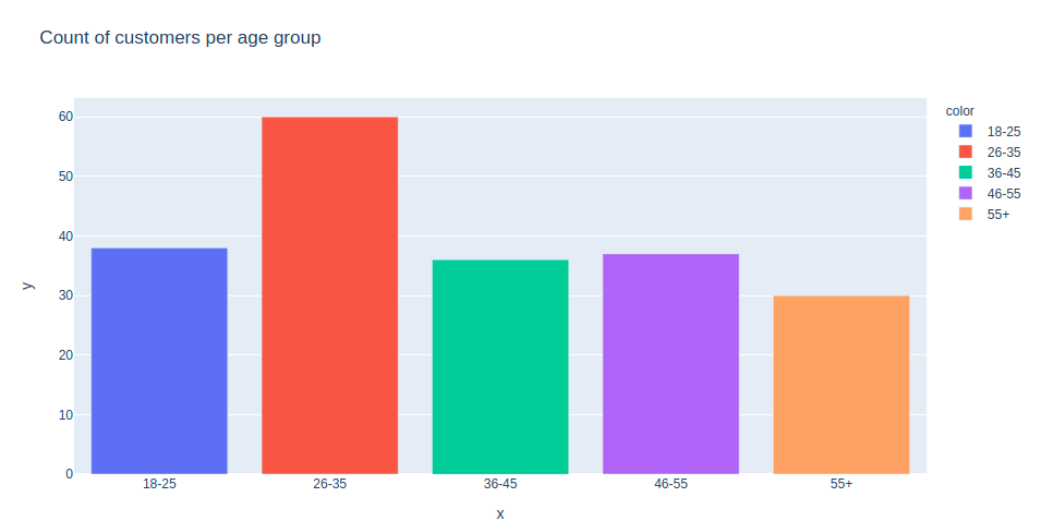
Now let’s create a bar plot to check the distribution of customers in particular age groups. You can also apply the same to visualize the number of customers versus spending scores and the number of customers based on their annual income.

age_55above = data.Age[data.Age >= 55]
age_46_55 = data.Age[(data.Age >= 46) & (data.Age <= 55)]
age_36_45 = data.Age[(data.Age >= 36) & (data.Age <= 45)]
age_26_35 = data.Age[(data.Age >= 26) & (data.Age <= 35)]
age_18_25 = data.Age[(data.Age >= 18) & (data.Age <= 25)]

x_age_ax = ['18-25', '26-35', '36-45', '46-55', '55+']
y_age_ax = [len(age_18_25.values), len(age_26_35.values), len(age_36_45.values), len(age_46_55.values),
     len(age_55above.values)]

pxp.bar(data_frame = data, x = x_age_ax, y = y_age_ax, color = x_age_ax,
       title = 'Count of customers per age group')

One of the most critical aspects of clustering is selecting the correct value of K. Randomly selecting K might not be a favorable choice. We’ll be using the elbow method and silhouette score to choose the value of K.

In our case, from the below graph, it looks like the optimal value of K found from the elbow method is 4. We want to maximize the number of clusters and limit cases where each data point becomes its cluster centroid.

x_input = data.loc[:, ['Age', 'SpendingScore']].values
wcss = []
for k in range(1, 12):
    k_means = KMeans(n_clusters=k, init='k-means++')
    k_means.fit(x_input)
    wcss.append(k_means.inertia_)

plot.figure(figsize=(15,8))

plot.plot(range(1, 12), wcss, linewidth=2, marker='8')
plot.title('Elbow methodn', fontsize=18)
plot.xlabel('K')
plot.ylabel('WCSS')
plot.show()

Let’s check how the Silhouette coefficient looks for this particular implementation.

from sklearn.metrics import silhouette_score
label = k_means.predict(x_input)
# Calculating Silhouette score
print(f' Silhouette Score(n=4): {silhouette_score(x_input,
label)}')

From the plot below of Age versus SpendingScore, you can see that some clusters aren’t well-separated. The intracluster distance between clusters is almost insignificant, and that’s why SC for n=4 is 0.40, which is less. Try different values of K to find the optimal number of clusters.

k_means=KMeans(n_clusters=4)
labels=k_means.fit_predict(x_input)
print(k_means.cluster_centers_)

Now let’s plot a graph to check how the clusters are formed from the data.

plot.figure(figsize = (16, 10))
plot.scatter(x_input[:, 0], x_input[:, 1], c =
k_means.labels_, s = 105)
plot.scatter(k_means.cluster_centers_[:, 0],k_means.cluster_centers_[:, 1], color = 'red', s = 250)
plot.title('Customers clustersn', fontsize = 20)
plot.xlabel('Age')
plot.ylabel('Spending Score')
plot.show()

Red dots indicate cluster centers.

The data forms four different clusters. The blue cluster represents young customers with bigger spending scores, and the purple cluster represents older ones with lower spending scores.

Similar steps implemented above can be followed to cluster `Age` versus `AnnualIncome`, and `SpendingScore` versus `AnnualIncome`. All three can be combined and plotted using a 3D plot that can be found in the Jupyter Notebook. It also has different clustering algorithms implemented on the same data.

2. Image compression

Image compression is a type of compression technique applied to images without degrading the quality of the picture. The reduction of image size helps store them in a limited amount of drive space.

Why are image compression techniques needed? There are a variety of needs for image compression. Compression is crucial in healthcare, where Medical images need to be archived, and the data volume is enormous. 

When we need to extract and store the most useful components of an image, represented as embeddings, image compression might be a very beneficial approach to storing more data.

There are two kinds of image compression techniques:

1. Lossless compression: This method is used to reduce the size of the file while maintaining the same quality as before it was compressed. The file can be restored to its original form, as this technique doesn’t compromise data quality.
2. Lossy compression: Lossy compression is a method that eliminates data that’s not noticeable. It gives the photo an even smaller size; lossy compression discards some less critical parts of the picture. In this type of compression technique, the compressed image cant be restored to its original image, and the size of the data changes.

Let’s use K-Means clustering to tackle this problem.

As you might already know, an image consists of 3 channels, RGB, each having values in the range [0, 255]. Thus a particular image might have 255*255*255 different colors. So before we feed the image, we need to preprocess it.

The size of the image that we will be working on is (1365, 2048, 3). So for each pixel location, we would have two 8-bit integers specify the red, green, and blue intensity values. Our aim here is to reduce it to 25 colors and represent the photo using those colors only.

Some of the packages required for this task are imported below:

import matplotlib.pyplot as plt
from matplotlib.image import imread
import pandas as pd
import numpy as np
import seaborn as sns
from sklearn.cluster import KMeans

Download the image from here and read it in.

img = imread('palace.jpg')
img_size = img.shape

Reshape the image to 2D. We apply the K-Means algorithm to the picture and treat every pixel as a data point to pick what colors to use. This means reshaping the image from height x width x channels to (height X width) x channel; we would have 1365 x 2048 = 2795520 data points. 

Following this method will help us represent the image using 25 centroids and reduce the image size. There will be a considerable difference where we’ll be using centroids as a look-up for the pixel colors, and that would reduce the size of each pixel location to 4-bit instead of 8 bit.

X = img.reshape(img_size[0] * img_size[1], img_size[2])

Run the K-means algorithm

A detailed explanation for the K-means algorithm is given in the above section. In this example, we’ll focus on the compression part.

km = KMeans(n_clusters=25)
km.fit(X)

Use centroids to compress the image.

X_cmpresd = km.cluster_centers_[km.labels_]
X_cmpresd = np.clip(X_cmpresd.astype('uint8'), 0, 255)

Reshape X_cmpresd to have the same dimension as the original image 128 * 128 * 3

X_cmpresd = X_cmpresd.reshape(img_size[0], img_size[1], img_size[2])

Now, plot the original and the compressed image next to each other.

figre, axs = plt.subplots(1, 2, figsize = (14, 10))
axs[1].imshow(img)
axs[1].set_title('Initial image')
axs[0].imshow(X_cmpresd)
axs[0].set_title('Compressed one (25 colors)')
for axs in figre.axes:
    axs.axis('off')
plot.tight_layout();

Here, I have used 25 centroids. A compressed image looks closer to the original one (meaning many characteristics of the real image are retained). With the smaller number of clusters, we would have a higher compression rate at the cost of image quality. Similar colors are grouped together into k clusters (k = 25(different RGB values)).

3. Digits classification

In this implementation, we’ll use Mini-Batch K-Means to perform image classification. Clustering can be used for image analysis as well. Utilizing Scikit-learn and the MNIST dataset, we’ll investigate the use of Mini-Batch K-Means clustering for computer vision.

Install dependencies:

pip install keras tensorflow

Import libraries:

import sys
import sklearn
import matplotlib
import numpy as np
import matplotlib.pyplot as plt
%matplotlib inline

Load the MNIST dataset. It’s available through Keras.

figur, axi = plt.subplots(3, 3, figsize=(14, 14))
plt.gray()

for j, axs in enumerate(axi.flat):
    axs.matshow(x_train[j])
    axs.axis('off')
    axs.set_title('number {}'.format(y_train[j]))

figur.show()

Preprocessing the images

Images stored as Numpy arrays are 2-D arrays. Mini-Batch K-means clustering algorithm provided by Scikit-learn ingests 1D arrays. As a result, we need to reshape the image. MNIST contains 28 x 28-pixel images; as a result, they will have a length of 784 once we shape them to the 1D array.

# Convert the image into 1 Darray
X = x_train.reshape(len(x_train), -1)
Y = y_train
# normalize the data
X = X.astype(float) / 255.
print(X.shape)
print(X[0].shape)

Clustering

Because of the size of the dataset, we’re using a Mini-Batch implementation of K-Means. The algorithm takes less time to fit the data.The MNIST dataset contains images of the integers 0-9. So, let’s start clustering by setting the number of clusters to 10.

from sklearn.cluster import MiniBatchKMeans
n_digits = len(np.unique(y_test))
print(n_digits)
# Initialize KMeans model
kmeans = MiniBatchKMeans(n_clusters=n_digits)
# fit the model
kmeans.fit(X)
kmeans.labels_

Assign cluster labels

Mini-Batch K-means is an unsupervised ML method meaning that the labels assigned by the algorithm refer to the cluster each array was assigned to, not the actual target integer. To fix this, let’s define functions that will predict which integer corresponds to each cluster.

def cluster_labels_infer(kmeans, actual_lbls):
    """
    returns: dictionary(clusters assigned to labels)
    """
    infrd_labels = {}
    for n in range(kmeans.n_clusters):
        labels = []
        index = np.where(kmeans.labels_ == n)
        labels.append(actual_lbls[index])

        # find common label
        if len(labels[0]) == 1:
            counts = np.bincount(labels[0])
        else:
            counts = np.bincount(np.squeeze(labels))

        # assigning cluster to a val in dict
        if np.argmax(counts) in infrd_labels:

            infrd_labels[np.argmax(counts)].append(n)
        else:
            # create a new array
            infrd_labels[np.argmax(counts)] = [n]

    return infrd_labels

def data_labels_infer(X_labels, clstr_labels):
    """
    Depending on the cluster assignment find the label
    predicted labels are returned for each array
    """
    pred_labels = np.zeros(len(X_labels)).astype(np.uint8)

    for l, clstr in enumerate(X_labels):
        for key, val in clstr_labels.items():
            if clstr in val:
                pred_labels[i] = key

    return pred_labels

Let’s test the functions written above to predict which integer corresponds to each cluster.

# test the functions written above
clstr_labels = cluster_labels_infer(kmeans, Y)
input_clusters = kmeans.predict(X)
pred_labels = data_labels_infer(input_clusters, clstr_labels)

print(pred_labels[:20])
print(Y[:20])

Evaluating and optimizing the clustering algorithm

With the functions returned above, we can determine the accuracy of our algorithm. Since we’re using clustering algorithms for classification, accuracy becomes an important metric. Some metrics can be applied to the clusters directly, regardless of associated labels. The metrics used are:

• Inertia
• Homogeneity

Previously, we made assumptions while choosing a particular value for K, but it might not always be the case. Let’s fit the Mini-Batch K-Means algorithm to different values of K and evaluate the performance using our metrics. The function to calculate metrics for a model is defined below.

from sklearn import metrics

def calculate_metrics(estimator, data, labels):

    # Calculate  metrics
    print('Number of Clusters: {}'.format(estimator.n_clusters))
    print('Inertia: {}'.format(estimator.inertia_))
    print('Homogeneity: {}'.format(metrics.homogeneity_score(labels, estimator.labels_)))

Now that we’ve defined metrics, let’s run the model for different numbers of clusters.

clusters = [10, 16, 36, 64, 144, 256]

# test different numbers of clusters
for n_clusters in clusters:
    estimator = MiniBatchKMeans(n_clusters = n_clusters)
    estimator.fit(X)

    # print cluster metrics
    calculate_metrics(estimator, X, Y)

    # determine predicted labels
    cluster_labels = cluster_labels_infer(estimator, Y)
    predicted_Y = data_labels_infer(estimator.labels_, cluster_labels)

    # calculate accuracy
    print('Accuracy: {}n'.format(metrics.accuracy_score(Y, predicted_Y)))

Let’s run the model in the test set with 256 as the number of clusters, as it has more accuracy for that particular number.

# testing
# convert each image to 1 D array
X_test = x_test.reshape(len(x_test),-1)
# normalize the data to 0 - 1
X_test = X_test.astype(float) / 255.
# fit KMeans algorithm
kmeans = MiniBatchKMeans(n_clusters = 256)
kmeans.fit(X)
cluster_labels = cluster_labels_infer(kmeans, Y)
# predict
test_clusters = kmeans.predict(X_test)
predicted_labels = data_labels_infer(kmeans.predict(X_test),
cluster_labels)
# calculate accuracy
print('Accuracy: {}n'.format(metrics.accuracy_score(y_test,
predicted_labels)))

Visualizing cluster centroids

The centroid is the point that is representative in every cluster. If we were dealing with A, B points, the centroid would simply be a point on the graph. Since we’re using an array of length 784, our centroid will also be an array of length 784. We can reshape this array back into a 28×28 pixel image and plot it.

#fit KMeans algorithm
kmeans = MiniBatchKMeans(n_clusters = 36)
kmeans.fit(X)

# record centroid values
centroids = kmeans.cluster_centers_

# reshape centroids into images
images = centroids.reshape(36, 28, 28)
images *= 255
images = images.astype(np.uint8)

# determine cluster labels
cluster_labels = cluster_labels_infer(kmeans, Y)

# subplots 
fig, axs = plt.subplots(6, 6, figsize = (20, 20))
plt.gray()

# loop through subplots and add centroid images
for i, ax in enumerate(axs.flat):

 # determine inferred label using cluster_labels dictionary
    for key, value in cluster_labels.items():
        if i in value:
            ax.set_title('Inferred Label: {}'.format(key))

    # add image to subplot
    ax.matshow(images[i])
    ax.axis('off')

# display the figure
fig.show()

These graphs display the most representative image for the cluster.

As the number of clusters and the number of data points increase, the relative saving in computational time increases. The saving in time is more noticeable only when the number of clusters is enormous. The effect of batch size in computational time is also more noticeable only when the number of clusters is larger. 

An increase in the count of clusters decreases the similarity of the Mini-Batch K-Means solution to the K-Means solution. As the number of clusters increases, the agreement between partitions decreases. This means the final partitions are different but closer in quality.

Clustering metrics

There are certain evaluation metrics to check how good the clusters obtained by your clustering algorithm are.

Homogeneity score

Homogeneity metric: Clustering results satisfy homogeneity if all its clusters contain only data points that are members of a single class. This metric is independent of the absolute value of labels. It’s defined as:

The homogeneity score is bounded between 0 and 1. A low value indicates low homogeneity, and 1 stands for perfectly homogeneous labeling. 

When the knowledge of Ypred reduces the uncertainty of Ytrue, becomes smaller (h → 1) and vice versa.

Perfect labelings are homogeneous. Non-perfect labelings that further split classes into more clusters can be homogeneous. Samples included from different classes in a cluster don’t satisfy homogeneous labeling.

Completeness score

Clustering results satisfy completeness only if the data points of a given class are part of the same cluster.

This metric isn’t symmetric, so switching label_true and label_pred from the above equation will return a homogeneity score which will be different. The same applies to the Homogeneity score; switching label_true and label_pred will return the completeness score.

Perfect labelings are complete. Non-perfect labelings that assign all class members to the same clusters are still complete. If class members are split across different clusters, the assignment can’t be complete.

V measure score

V-measure cluster labeling gives a ground truth. The V measure is the harmonic mean between homogeneity and completeness.

This metric is symmetric. Switching `label_true` with `label_pred` will return the same value. When the real ground truth is unknown, this metric can be helpful to calculate the acceptance of the two independent label assignment techniques on the same dataset.

The score ranges between 0-1. 1 stands for perfectly complete labeling.

Example:

from sklearn import metrics
true_labels = [2, 2, 3, 1, 1, 1]
pred_labels = [1, 1, 2, 3, 3, 3]
metrics.homogeneity_score(true_labels, pred_labels)
Output: 1.0

metrics.completeness_score(true_labels, pred_labels)
Output: 1.0

(1 stands for perfectly complete labeling)
metrics.v_measure_score(true_labels, pred_labels)
Output: 1.0
-------------------------------------------------------------------
true_labels = [2, 2, 3, 6, 1, 1]
pred_labels = [1, 1, 2, 3, 2, 1]
metrics.homogeneity_score(true_labels, pred_labels)
Output: 0.58688267143572
metrics.completeness_score(true_labels, pred_labels)
Output: 0.7715561736794712
metrics.v_measure_score(true_labels, pred_labels)
Output: 0.6666666666666667

Adjusted rand score

The similarity between two clusters can be calculated using the Rand Index(RI) by counting all pairs of samples and counting pairs assigned in different or same clusters in the true and predicted clusters. The RI score is then “adjusted for chance” into the ARI score using the following scheme.

ARI is a symmetric measure:

Please refer to the link for a detailed user guide

Adjusted Mutual Info Score

Adjusted Mutual Information(AMI) score is an adjustment for the Mutual Information Score to account for a chance. It accounts for the fact that the Mutual Information Score is generally higher for 2 clusters with many clusters, regardless of whether there’s more information shared. 

For two clusterings U and V, the AMI is given as:

For a user guide, please refer to the link. The GitHub repo has the data and all notebooks for this article.

Summary

This blog covered the most critical aspects of clustering, image compression, digit classification, customer segmentation, implementation of different clustering algorithms, and evaluation metrics. Hope you guys learned something new here.

Thanks for reading. Keep learning!

Reference

1. https://scikit-learn.org/stable/modules/clustering.html
2. https://towardsdatascience.com/the-5-clustering-algorithms-data-scientists-need-to-know-a36d136ef68
3. https://medium.datadriveninvestor.com/k-means-clustering-for-imagery-analysis-56c9976f16b6
4. https://imaddabbura.github.io/post/kmeans-clustering/
5. https://www.geeksforgeeks.org/ml-mini-batch-k-means-clustering-algorithm/
6. https://scikit-learn.org/stable/modules/generated/sklearn.metrics.v_measure_score.html#sklearn.metrics.v_measure_score
7. https://www.kaggle.com/niteshyadav3103/customer-segmentation-using-kmeans-hc-dbscan
8. https://www.linkedin.com/pulse/gaussian-mixture-models-clustering-machine-learning-cheruku/