
The first computer bug was literally a bug. A moth entered one of the computing machines at Harvard University in 1947 and caused a disruption in the computations. When engineers opened the computer box, they quickly detected the bug that was causing the problems. Nowadays, it is very unlikely that a bug will crawl into our computer and disrupt the computational flow. However, the principle remains the same.
A software bug is a small, hard-to-notice error that creeps into our software project and causes problems. Unfortunately, unlike spotting a moth, software bugs are more subtle and difficult to detect. In most cases, software developers create those bugs by making small errors in their code that at first appear innocent. This is the reason for the existence of many tools and approaches that aid programmers in debugging their code.
In this article, I’ll dive deeper into the topic of debugging deep learning models and explain how to do it.

What is deep learning model debugging and why is it different from software debugging?
In software debugging, programmers follow a predefined set of rules that allow them to reach the root of the problem. In a sense, it is similar to following a white pebbles trail like the ones created by Hansel and Gretel. In software debugging, the art is where exactly to leave the white pebbles such that bugs can be detected easily.
Machine learning is however different. We are not simply solving a well-defined task that has a deterministic output for a given input. We are training a model that captures the structure of data from a given domain such that the algorithms learn to recognize patterns that can be used to predict the behavior of future examples. The implementation of the model might not have any software bugs, yet the model can be buggy. As an example, consider a model that has been trained using incorrectly preprocessed data. Clearly, this is a serious limitation and the model needs to be retrained. However, from a software point of view, there is nothing wrong with the model, it works correctly for the provided input.
The more powerful the model the more sophisticated the bugs.
The above is particularly true for deep learning. One can argue that the main advantage of deep learning models is their ability to learn relevant features from data. While this yields powerful models, it is also a challenge. Just like interpretability is a serious issue for deep learning, debugging can be particularly challenging. Consider again the example with wrongly preprocessed input. For instance, we have converted the colors of the input images by using signed instead of unsigned integers. A CNN model will learn how to work with the wrong input and still achieve excellent results. But when evaluated on new, correctly preprocessed data, the algorithm will fail.
In this article, we concentrate on debugging deep learning models. Arguably, neural networks yield the most advanced prediction models. At the same time, they are the most challenging models in terms of design, debugging, and maintenance. We will discuss the challenges and present strategies to cope with those challenges.
You might have missed
In-depth Guide to ML Model Debugging and Tools You Need to Know
Best Practices for Improving Your Machine Learning and Deep Learning Models
How to debug deep learning models?
The design of a neural network based model should go hand in hand with strategies for its debugging. We list the basic steps that should always be followed when working on the implementation and evaluation of a deep learning model.
1. Debug the implementation
Software bugs might be hidden by the power of deep learning. For example, we have the following implementation of a convolutional neural network in Keras:
inp = Input(shape=(28, 28, 1))
x = Conv2D(32, kernel_size=(3, 3), activation="relu")(inp)
x = MaxPooling2D(pool_size=(2, 2))(x)
x = Conv2D(32, kernel_size=(3, 3), activation="relu")(x)
x = MaxPooling2D(pool_size=(2, 2))(x)
…
For the second convolutional layer, we are likely to copy the code that we used for the first one, namely x = Conv2D(32, kernel_size=(3, 3), activation=”relu”)(inp), and forget to update the input to x. The model will still work, it will just be a simpler model than the one we actually wanted to implement.
Tip: Create tests that assert that the neural network architecture looks the way it is supposed to, checking the number of layers, the total number of trainable parameters, the value range of the output, and so on. Ideally, visualize the network architecture like shown in Figure 2.

2. Check the input
Simple errors like providing our model with a subset of the features due to wrong indexing might be hard to detect. A deep learning model will still work, even if provided with fewer features. More generally, the power of deep learning might turn out to be a curse if we make a systematic error when preprocessing the input data. The model will adapt itself to the incorrect input and then it will not work properly once we have fixed our preprocessing bug.
Tip: Implement tests that assert the format and the values range of the input features.
3. Initialize carefully the network parameters
Before starting training, we have to initialize the parameters of our model. Most likely, we use an available platform TensorFlow or PyTorch that will take care of initialization. However, errors at this stage are still possible as the parameters are selected according to the number of inputs and outputs for each neuron. Here is Andrej Karpathy’s advice on initialization.
Look for correct loss at chance performance. Make sure you’re getting the loss you expect when you initialize with small parameters. It’s best to first check the data loss alone (so set regularization strength to zero). For example, for CIFAR-10 with a Softmax classifier we would expect the initial loss to be 2.302, because we expect a diffuse probability of 0.1 for each class (since there are 10 classes), and Softmax loss is the negative log probability of the correct class so: -ln(0.1) = 2.302.
Tip: More generally, write tests that assert the input before training yields expected results. In the above example, we can assert that the entropy for the probability distribution for k predicted classes is close to -k ln 1/k = k ln k.
4. Start simple and use a baseline
Observe that several basic models can be implemented using a neural network. For example, we can implement linear regression as a shallow network with mean squared error as the loss function. Similarly, logistic regression can be implemented by a shallow network with a sigmoid activation function for the output and binary cross-entropy as the loss function. Figure 3 shows a logistic regression model by removing the hidden layers from the network in Figure 2:

where w1 to wn are the learnable parameters.
Also, we can simulate PCA using an autoencoder with linear activation functions. Thus, it is a good idea to compare the results of our neural network implementation for a basic algorithm to the result we obtain from a publicly available implementation in a platform like scikit-learn of the same algorithm. This would allow us to catch different kinds of errors early on, such as weight initialization errors, learning rate problems, wrong input preprocessing, etc.

Tip: Write tests that assert that the results for the same input of our deep learning implementation and some off-the-shelf algorithms are comparable.
5. Check intermediate outputs
We can think of deep learning models as a concatenation of (non-linear) functions. Consecutive layers compute more and more complex features. Thus, we can track these new features. This is particularly intuitive for deep convolutional neural network models where the features computed by each layer can be visualized.
Similar to standard software debugging, where we set breakpoints that allow us to track the intermediate values assigned to the variables in our program, we can also track the intermediate outputs of our deep learning model.
In particular, we can use a debugging tool.
Tip: Write tests that check the output values after each layer. Also, use visualization tools that show the different layers of the model.
6. Make sure that our model is properly designed
You should specifically pay attention to:
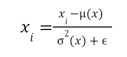
- Feature normalization. It is important that input features are of the same magnitude, thus for features of different scales it is important to use an appropriate normalization technique. Popular choices are standardization and min-max normalization:
- Standardization
- Min-max normalization
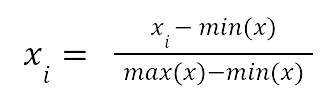
In the above, x is the input vector and the xi are the individual coordinates.
- Prevent vanishing gradients. For certain loss functions, we might encounter the problem of vanishing gradients. The gradient at each layer is multiplied by the gradients at subsequent layers. Consider the sigmoid function σ(z) = 1/(1+e-z). For large or small values of z the gradient will be close to 0, thus we should be careful when using it as an activation function. The rule of thumb is to use sigmoid, or more generally softmax, only for the output layer.
Tip: The tests that check the output at each layer, should check for output that is close to 0 at intermediate layers.
Might be useful
How to Monitor, Diagnose, and Solve Gradient Issues in Foundation Models
- Batch size. It is standard to use the mini-batch approach when training a neural network. In this setting, we use subsamples of the data for which we compute the loss and update the parameters of the networks using gradient descent computed by backpropagation. Of course, the exact size of the mini-batch depends on the computation hardware constraints and the dataset size. It holds that a small mini-batch size will lead to many training epochs while a larger mini-batch size will cause slow training.
- Batch normalization. We normalize the input to each layer by normalization of each input feature. Here it is important to remember that the mean and variance are computed for each mini-batch but during inference, they are computed for the whole training dataset. (We might want to evaluate the model for a single example.)
Tip: Write tests that ensure that the inputs for each layer are indeed normalized.
- Oscillation around the optimal value. The learning rate needs to be adapted in order to address changes in the curvature for complex functions. In particular, the gradients in different directions might be of largely different magnitude, thus using a constant learning rate might lead to oscillations. A popular choice in practice is the Adam approach (Adaptive Moment Estimation) where the learning rate is adjusted after each iteration by using an exponentially decreasing average of past gradients.

7. Prevent overfitting
Another important point to remember is that the model should be able to generalize to new data. The power of neural networks might easily lead to overfitting such that we learn noise in the input instances. Here we list some of the commonly used regularization techniques.
- Node weight regularization. It is standard to use weight regularization that prevents certain weights from becoming too large and thus overfitting the input. The standard choices are L1 and L2 regularization: we add to the loss function a term λ||W||p where W are the learnable weights of the model and >0 is the strength of the regularization.
- Dropout. During training, we randomly delete a fraction of the neurons in a given layer. This prevents neurons from becoming overspecified and learning very particular patterns that are more likely random artifacts.
- Early stopping. When designing the model, we evaluate its performance on a subset of the data that has not been used for training, the so-called validation data. We stop training the model once the performance on the validation does not seem to improve for a certain number of epochs.
- Data augmentation. In order to force the model to learn only the significant patterns in the data, we can generate some artificial data by augmenting our dataset. For computer vision applications we can rotate or mirror the input images, or change the colors such that the generated new data still looks like natural images, see Figure 5 for an example.. Keep in mind that data augmentation can be challenging for certain domains and we should be careful when applying it such that we don’t create a bias in the training data.


8. Document and track experiments
Neural networks use different kinds of randomization in order to train high-quality models. The weights of internal layers are initialized by random weights according to different strategies, we might use dropout for regularization, or we might use cross-validation when designing the model.
Tip: Use a random seed and store the randomization choices.
The above will make the neural training process reproducible and will simplify the detection of bugs. In particular, certain problems might be caused by differences in the underlying hardware and this can be detected by reproducing the complete training flow.
Learn more
ML Experiment Tracking: What It Is, Why It Matters, and How to Implement It
9. Be patient
Always keep in mind that deep learning model training is a slow and often painful process. Sometimes we might obtain results that were not really expected but this does not necessarily mean there is a problem with our model. For example, consider this reddit discussion that has gained some popularity. As Andrej Karpathy reports:
“One time I accidentally left a model training during the winter break and when I got back in January it was state of the art.”
Waiting for hours until our model performance starts to improve might appear counterintuitive and does not happen very often, in fact early stopping is based on the premise that this is not really feasible. But it is not necessarily an indication of a problem with our model. At a high level, deep learning models search for the optimal set of parameters with respect to a given objective. And optimizing with respect to this objective is not a well-defined task but rather a heuristic based on the concept of backpropagation that guarantees to find a local optimum for the loss function in question. However, a non-convex function with thousands of parameters is likely to have many local minima.
Thus, there are instances where the search might converge to an exhaustive search of the function parameter space and appear as making no progress. In a recent paper, researchers have designed a set of learning problems for which the learning is guaranteed to take long before finding an optimal solution. In fact, overfitting on the training data is necessary such that an optimal solution is found. Of course, this is an artificial setting and real-life data is very unlikely to exhibit the same behavior. But we should keep in mind that detecting complex patterns might take longer than our intuition tells us and devote some time to check if this is not the case with our model.

Tip: When planning work on the model development, leave enough time for the model to train in order to make sure we won’t experience a sudden decrease in the loss function.
Conclusions
Debugging neural network models can be a challenging task that might require profound understanding and experience in different areas of software development and machine learning techniques. Before designing a neural network solution, it is therefore important to have a well-defined strategy that will simplify model debugging. Having a plan on how to deal with potential problems will not only add to the robustness of the model but might also lead to new insights and a more powerful model.
Resources
- Amazon SageMaker Debugger – The debugger for models created by Amazon SageMaker.
- TensorWatch – A visual debugging tool by Microsoft
- TensorBoard – TensorFlow’s visualization tool.
- Neptune for Experiment Tracking
- DeepKit – An open-source platform for testing and debugging ML models.
- TensorFlow Debugger – Provides features to inspect the flow of the learning process during runtime.
- Debugging Machine Learning Models – Workshop at ICLR 2019
