Imbalanced Data in Object Detection Computer Vision Projects

One of the typical issues faced by data science practitioners is the data imbalance problem. It plagues every other ML project and we all have faced it while working on some classification problem. 

There can be several types of data imbalances. For instance, one of the most frequently discussed problems is class imbalance. While collecting real-world data, the possibility of having a dataset with balanced classes is really low. The class with a higher number of data points would tend to create a bias in the model and these biased models can be misinterpreted as performing well if you are using a simple accuracy score. 

Say, if in a test set, 97% of patients diagnosed do not have cancer, and 3% do. And our biased model is predicting none of the patients to have cancer, the accuracy would be 97%. So correct accuracy metrics is one of the important aspects of dealing with class imbalance problems. 

Similarly, there can be other kinds of imbalances that may occur in datasets depending on the nature of the problem and the rawness of the dataset. In this article, we’ll look at these different imbalances in the context of object detection problems and how to solve them.

Read also

How to Deal With Imbalanced Classification and Regression Data

Object Detection Algorithms and Libraries

Imbalance in object detection models

Object detection is simultaneously locating the object of interest in a picture while categorizing it into a certain class. The first generation of object detection algorithms mostly relied on hand-crafted features and linear classifiers, before deep learning came into the picture. With deep learning, while object detection achieved significant improvement, new problems arose i.e. imbalance problems.

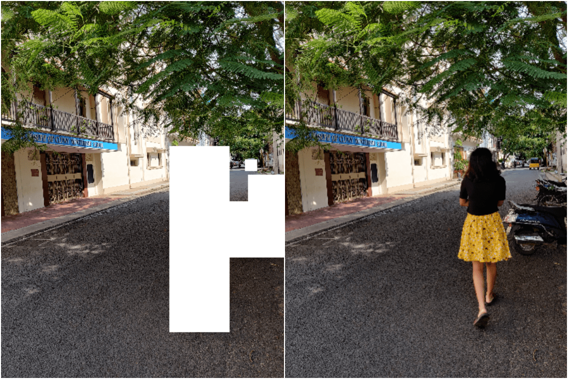
There are several input properties in an image, like different objects in images, area of foreground, and background, the contribution of different tasks (like classification and regression in a network), etc. If the distribution of these properties is not uniform, it results in imbalance problems. Figure 1 is an example of an Imbalance in the Data for Object Detection Model.

Now let’s discuss these different types of imbalances in Object detection in detail.

Class imbalance

If the number of instances for one object is more than another across the dataset, it results in class imbalance. In object detection, we can classify the area in an image into foreground and background, as can be seen in Figure 2.

Class imbalance from an object detection point of view can be subclassified into two types – foreground-background imbalance and foreground-foreground imbalance.

1. Foreground-Background Imbalance

In general, the area of background is much more than that of the foreground, hence most bounding boxes are labeled as background.

You can see a huge difference between background and foreground anchors in Figure 3. Now, this can easily result in a biased model giving more false negatives.

2. Foreground-Foreground Imbalance

Background anchors are not objects of interest in this case. In images, some objects can be overrepresented, whereas others can be underrepresented. Hence, when one class dominates the other, this is called foreground-foreground Imbalance. For example in figure 1, the number of vehicles dominates the number of people.

In figure 4 we can observe foreground-foreground imbalance.

Solving class imbalance

There are several effective ways to handle this problem. Let’s start with the most straightforward method.

1. Hard Sampling

Hard sampling is directly dropping certain bounding boxes, such that they have no effect on the training, there are different heuristical ways to do so.

So if w is the weight given to sample, w will define its contribution to training. For hard sampling, either w=0 or w=1.

• Random Sampling

While training, from a batch for each image, a certain number of negative and positive samples are selected, and the rest are dropped.

• Hard Negative Mining

Instead of randomly sampling, we pick the list of the negative samples from top to bottom (the topmost being the one with the most probability of being negative). We select negative examples (topmost) such that the negative to positive ratio issue is no more than 3:1. The hypothesis behind this method is that a training algorithm with more hard examples (which gives higher loss) results in better performance eventually.

• IoU Based Sampling

The negative samples are distributed to K bins, and then uniformly selected from each bin. This promotes samples with high IoUs which give a high loss value. This also follows the same hypothesis as hard negative mining.

2. Soft Sampling

Unlike Hard sampling where the weight of positive and negative samples is binarized(either they contribute or they don’t), in Soft Sampling, we adjust the contribution of each sample based on some methods. One of them is Focal Loss.

Using Focal loss is one of the bests methods for soft sampling and handling the class imbalance. It gives more weightage to hard samples.

FL(p_t) = -α(1-p_t)^λlog(p_t)

In the loss equation above, p_t is the estimated probability of the sample. Now if p_t≃1, loss would tend towards zero (FL≃0), hence considering only hard examples.

A good PyTorch implementation for Focal loss can be found here.

3. Generative Methods

Sampling methods decrease and increase the weights of samples. However generative methods can generate new artificial samples to balance the training. The dawn of Generative Adversarial Networks(GANs) gave a boost to this method.

May interest you

6 GAN Architectures You Really Should Know

Paper Adversarial Fast RCNN shows how it can be used in two stages. The images from the dataset are taken, and in two stages now transformed images are generated.

1. ASDN: Adversarial Spatial Dropout Network creates occlusion in images
2. ASTN: Adversarial Spatial Transform Network rotates the channels from -10deg to 10deg to create harder examples.

Figure 6 shows the areas occluded are of importance for classifier. Making these changes would allow generating more hard samples and a more robust classifier.

Official implementation of the paper in Caffe can be found here, it’s quite easy to follow.

The paper focuses on hard positive generation. But the Generative method can be used for foreground-background class imbalance as well.

Scale imbalance

Scale Imbalance is another critical problem faced while training object detection networks. Scale imbalance occurs because a certain range of object size or some particular level (high/low level) of features are over and under-represented.

Scale imbalance can be sub-classified into – box level scale imbalance or feature-level scale imbalance.

1. Box level scale imbalance

In a dataset distribution of certain objects, sizes can be over-represented. In such cases, the trained models can result in bad Regions of Interest biased towards the over-represented sizes.

Figure 7 clearly shows a higher frequency for small-sized objects.

2. Feature level scale imbalance

The imbalanced distribution of low-level and high-level features can create inconsistent predictions. Let’s take an example to understand this. Faster RCNN, a rather popular method of object detection uses a Feature pyramid network (FPN) for Region Proposal.

In figure 8, we see the basic architecture of FPN. When we pass the input image to the bottom-up pathway and convolution takes place, the initial layers consist of low-level features, and subsequent layers have more complex high-level features.

Note that each layer in the top-down pathway proposes regions of interest. So all the layers should have a balanced amount of low-level and high-level features. But that is not the case as we can see in the top-down pathway, we’ll have more high-level features in the topmost layer and more low-level features in the bottom-most layer. Hence, this could result in inconsistent predictions.

Solving scale imbalance

To solve scale imbalance, you would deal more with network architectural changes rather than changes in loss function as we did in class imbalance. We discussed two types of scale imbalance, let us see how to tackle them.

1. Box level scale Imbalance

As you can see in Figure 9, the earlier object detectors were used to predict regions of interest on the last layer, after all the convolution and pooling was done. This did not take in account the diversity of bounding boxes’ scales.

This is where the feature pyramid comes into play. FPN (Figure 8) includes bottom-up pathway, top-down pathway and lateral connections. It gives rich semantics from high to low levels.

FPN can be used wherever Region proposal networks are required. You can read more about FPN here.

In PyTorch, you can simply get FPN from torchvision.ops;

from torchvision.ops import FeaturePyramidNetwork
net = FeaturePyramidNetwork([10, 20, 30], 5)
print(net)

Output:

FeaturePyramidNetwork(
  (inner_blocks): ModuleList(
    (0): Conv2d(10, 5, kernel_size=(1, 1), stride=(1, 1))
    (1): Conv2d(20, 5, kernel_size=(1, 1), stride=(1, 1))
    (2): Conv2d(30, 5, kernel_size=(1, 1), stride=(1, 1))
  )
  (layer_blocks): ModuleList(
    (0): Conv2d(5, 5, kernel_size=(3, 3), stride=(1, 1), padding=(1, 1))
    (1): Conv2d(5, 5, kernel_size=(3, 3), stride=(1, 1), padding=(1, 1))
    (2): Conv2d(5, 5, kernel_size=(3, 3), stride=(1, 1), padding=(1, 1))
  )
)

There are different variants of FPN as well, which we’ll discuss in the next section.

2. Feature Level Scale Imbalance

We discussed before how FPN has shortcomings that lead to Feature level imbalance. Let’s look at one of the networks which helps solve this problem; Path Aggregation Network (PANet).

You can see the architecture of PANet here.

PANet has two components in addition to FPN, which generate enhanced features. The bottom-up path augmentation allows low-level features to be included in the prediction and the second is, that PANet associates RoIs to every level using adaptive feature pooling.

Spatial imbalance

There are certain spatial aspects of bounding boxes, which include, Intersection over Union (IoU), shape, size and location. It is obvious that in real-world examples, there would be an imbalance in such attributes, which would affect training. 

Now we’ll see how these different attributes of bounding boxes would affect training:

1. Imbalance in regression loss

Regression loss in an object detection network is usually used to tighten the bounding boxes of objects in an image. A small change in the position of the predicted bounding box and ground truth can cause a drastic change in regression loss. So it is very important to choose a stable loss function for regression which can handle this kind of imbalance.

In figure 11 we can observe how L1 and L2 loss behaves differently on the same IoU values.

2. IoU distribution Imbalance

When the distribution of IoU for bounding boxes (across the dataset) is skewed, it is called an IoU distribution Imbalance.

IoU distribution can affect two-stage networks as well, for example, when IoU distribution imbalance was dealt with in the second stage of faster RCNN, it showed significant improvement.

3. Object Location Imbalance

We use convolutional networks which follow the sliding window approach. Each window is assigned with certain scales of anchors, giving each window equal importance. However, the object location distribution across images is not uniform, thus causing the imbalance.

We can see in Figure 13, we can observe that object location distribution in the datasets is not uniform, but rather normal (gaussian).

Solving spatial imbalance

Let’s talk about solutions to all three imbalances in Spatial Imbalance one by one.

1. Imbalance in Regression Loss

Certain loss functions can help stablize regression loss. Look at the following table:

In the table, we can see different loss functions. I personally prefer smooth L1 Loss. It is robust and works well in most cases.

2. Imbalance in IoU Distribution

There are architectures that address the problem of IoU distribution Imbalance.

1. Cascade RCNN – Here the authors of the paper create three detectors in a cascaded pipeline with different IoU threshold. And the fact that each detector uses boxes from the previous stage instead of sampling them anew, shows that IoU distribution can be shifted from left-skewed to uniform and even right-skewed.
2. Hierarchical Shot Detector – Instead of using a cascaded pipeline, the network method runs its classifier after the boxes are regressed. This results in a more balanced IoU distribution. You can read the architecture in more detail in the paper.
3. IoU Uniform RCNN – This architecture adds variations in such a way it provides uniform bounding boxes to the regressor branch and not the classification branch.

All these networks have proved to be efficient in handling IoU distribution, increasing the overall performance of detection.

      3. Imbalance in Object Location

A Concept called Guided Anchoring deals with this problem to a certain extent. Here each of the feature maps from the feature pyramid is passed through the anchor guiding module before going to the prediction layers. The Guided Anchoring Module consists of two parts; the anchor generation part predicts the anchor shape and location, and the feature adaptation part applies new feature maps with anchor information to the original feature maps generated by the feature pyramid.

Objective imbalance

As we discussed before, for object detection there are two problems we need to optimize; classification and regression. Now calculating loss for both problems simultaneously can impose certain issues:

1. One of the tasks can dominate training due to the difference in the range of gradients.
2. Difference in loss range calculated in different tasks can be different. For example, a loss function converging for regression can be somewhere around 1, while for classification it can be around 0.01.
3. Difficulties of tasks can be different. For example, for a certain dataset reaching convergence for classification can be easier than regression.

Solving objective imbalance

1. CARL

An approach named Classification Aware Regression Loss (CARL) assumes Classification and Regression are correlated. 

L_C(x) = c_iL1_S(x)

Here L1S is the Smooth L1 loss being used as regression loss function. And ci is the classification factor based on the class probability calculated by classification layers. This way regression loss provides classification with gradient signals, thus deploying a correlation between Classification and Regression.

2. Guided Loss

The fact that regression loss consists of only foreground examples and is normalized only by the number of foreground classes, it can be used as a normalizer for the classification loss.

Guided loss weights the classification component by considering the total magnitude of the losses as –

wregLregLcls

Some useful tips and tricks

As we discussed earlier, the class imbalance is one of the biggest headaches while training an object detection model. Apart from changing the loss function and modifying the architecture, we can use some common sense and play around with the dataset to reduce the class imbalance. In this section, we’ll try to mitigate this issue through some data pre-processing.

Let’s consider an image (in figure 16) with geographic data. We want to identify objects like buildings, trees, cars, etc. The image in figure 16 is one of the images in the training dataset for our object detection network.

It is a high-resolution satellite picture. Now we are to identify buildings, cars, trees, etc. However, we can clearly see most of the picture consists of buildings. There’s a huge class imbalance as you’ll see in almost all real-life datasets. So how can we resolve this issue here?

To begin with, we could extract detailed images like figure 17 from it, if it’s of particularly high-resolution and then try any of the following approaches.

Merging classes

If possible merge similar classes. For example, if we have ‘cars’ and ‘trucks’ and ‘buses’ labeled in the dataset, merging them into the category ‘cars’ would increase the number of instances (for a label ‘cars’) and reduce the number of classes. The average pixel diameter of all three labels would be almost the same.

This is a simple and generic example, but ideally, this should be done by someone who has domain knowledge.

Splitting images

Instead of downscaling the high-resolution image, you can divide it into a certain number of tiles, and use each tile as input for the detection model. This would help the network learn smaller objects.

While downscaling will reduce the training time, it will also make small objects disappear. Tiling the dataset will certainly help.

import cv2
from matplotlib.pyplot import plt

a, b = 8, 10

img = cv2.imread('image_path')
M = img.shape[0]//a
N = img.shape[1]//b
tiles = [img[x:x+M,y:y+N] for x in range(0,img.shape[0],M) for y in range(0,img.shape[1],N)]

plt.imshow(tiles[0])

You can use this simple piece of code to split your images.

Under and oversampling

Under sampling and oversampling are the most basic methods of handling class imbalance. But in case, if you have enough time and data, you can try these things out.

Undersampling

Undersampling is when you discard datapoint from the overrepresented class. 

Now that you have made tiles in figure 18. You can discard tiles containing only buildings, this will balance the other objects, like canopy, cars, etc in your dataset.

The con is, that this can lead to a bad model. The buildings would be less generalized and when you infer on your model, there’s a possibility that it won’t recognize certain types of buildings.

Oversampling

In Over Sampling you generate synthetic data for underrepresented classes. We already saw an example in the section above on using generative algorithms like GANs. 

We can also oversample by simply using CV algorithms. For example, you have a tile filled with cars, you augment it but rotating, vertical and horizontal flipping, changing the contrast, adding wraps, shearing the image, etc.

We have transforms available in PyTorch, or you can just use OpenCV for such tasks.

The con to oversampling is, that your model can overfit your underrepresented data which you oversampled.

Bookmark for later

Building and Deploying CV Models: Lessons Learned From Computer Vision Engineer

Open issues and on-going research

Issues created by an imbalance in Deep Learning Networks is a fairly new topic of research, with more complex networks new imbalance problems are being identified more frequently.

In Regression loss imbalance we saw a lot of loss function solving issues for different kinds of problems, it is still an open issue and work is being done to integrate all the benefits of different loss functions into one.

There are a lot of examples like this where extra work is needed. There’s still no single unified method to handle all the different imbalances. Work on different architectures is ongoing.

The good thing is there are tons of resources to read about and tackle these imbalances.

Further reads

• Best work to put in one place the identified imbalances and their solutions: https://arxiv.org/pdf/1909.00169.pdf
• Github Repo pointing out all papers on imbalances in Object Detection: https://github.com/kemaloksuz/ObjectDetectionImbalance#2
• Good take on Focal loss: https://amaarora.github.io/2020/06/29/FocalLoss.html
• Adversarial Fast RCNN: https://arxiv.org/pdf/1704.03414.pdf