
Word embeddings is one of the most used techniques in natural language processing (NLP). It’s often said that the performance and ability of SOTA models wouldn’t have been possible without word embeddings. It’s precisely because of word embeddings that language models like RNNs, LSTMs, ELMo, BERT, AlBERT, GPT-2 to the most recent GPT-3 have evolved at a staggering pace.
These algorithms are fast and can generate language sequences and other downstream tasks with high accuracy, including contextual understanding, semantic and syntactic properties, as well as the linear relationship between words.
At the core, these models use embedding as a method to extract patterns from text or voice sequences. But how do they do that? What is the exact mechanism and the math behind word embeddings?
In this article, we’ll explore some of the early neural network techniques that let us build complex algorithms for natural language processing. For certain topics, there will be a link to the paper and a colab notebook attached to it, so that you can understand the concepts through trying them out. Doing so will help you learn quicker.
Topics we’ll be covering:
- What are word embeddings?
- Neural Language Model
- Word2Vec
- Skipgrams
- Continuous bag of words
- On softmax function
- Improving approximation
- Softmax-based approaches
- Hierarchical Softmax
- Sampling-based approaches
- Noise contrastive estimation
- Negative sampling
- Softmax-based approaches
What are word embeddings?
Word embeddings are a way to represent words and whole sentences in a numerical manner. We know that computers understand the language of numbers, so we try to encode words in a sentence to numbers such that the computer can read it and process it.
But reading and processing are not the only things that we want computers to do. We also want computers to build a relationship between each word in a sentence, or document with the other words in the same.
We want word embeddings to capture the context of the paragraph or previous sentences along with capturing the semantic and syntactic properties and similarities of the same.
For instance, if we take a sentence:
“The cat is lying on the floor and the dog was eating”,
…then we can take the two subjects (cat and dog) and switch them in the sentence making it:
“The dog is lying on the floor and the cat was eating”.
In both sentences, the semantic or meaning-related relationship is preserved, i.e. cat and dog are animals. And the sentence makes sense.
Similarly, the sentence also preserved syntactic relationship, i.e. rule-based relationship or grammar.
In order to achieve that kind of semantic and syntactic relationship we need to demand more than just mapping a word in a sentence or document to mere numbers. We need a larger representation of those numbers that can represent both semantic and syntactic properties.
We need vectors. Not only that, but learnable vectors.
In a mathematical sense, a word embedding is a parameterized function of the word:
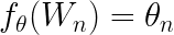
where is the parameter and W is the word in a sentence.
A lot of people also define word embedding as a dense representation of words in the form of vectors.
For instance, the word cat and dog can be represented as:
W(cat) = (0.9, 0.1, 0.3, -0.23 … )
W(dog) = (0.76, 0.1, -0.38, 0.3 … )
Now, hypothetically speaking, if the model is able to preserve the contextual similarity, then both words will be close in a vector space.

So far we’ve dealt with two words (cat and dog), but what if there are more words? The job of a work embedding model is to cluster similar information and establish a relationship between them.
As you can see, word embeddings clusters similar words together.

There are a lot of shallow algorithms present that work well for clustering. Why do we need neural networks?
One of the biggest misconceptions is that word embeddings require deep neural networks. As we build different word embedding models, you will see that for all the embeddings, the model is a shallow neural network, and some are linear models as well.
The reasons we use neural networks to create word embeddings are:
- It’s useful in finding nearest neighbors in the embedding space.
- It can be used as an input to supervised learning tasks.
- It creates a mapping of discrete variables, such as words to a vector, of continuous variables.
- It also tackles the curse of dimensionality.
Learn more
Training, Visualizing, and Understanding Word Embeddings: Deep Dive Into Custom Datasets
Neural Language Model
Word embeddings were proposed by Bengio et. al. (2001, 2003) to tackle what’s known as the curse of dimensionality, a common problem in statistical language modelling.
It turns out that Bengio’s method could train a neural network such that each training sentence could inform the model about a number of semantically available neighboring words, which was known as distributed representation of words. The neural network not established relationships between different words, but it also preserved relationships in terms of both semantic and syntactic properties.

This introduced a neural network architecture approach that laid the foundation for many current approaches.
This neural network has three components:
- An embedding layer that generates word embedding, and the parameters are shared across words.
- A hidden layer of one or more layers, which introduces non-linearity to the embeddings.
- A softmax function that produces probability distribution over all the words in the vocabulary.
Let’s understand how a neural network language model works with the help of code.
(here are links to the Notebook and original Paper)
Step 1: Indexing the words. We start by indexing the words. For each word in the sentence, we’ll assign a number to it.
word_list = " ".join(raw_sentence).split()
word_list = list(set(word_list))
word2id = {w: i for i, w in enumerate(word_list)}
id2word = {i: w for i, w in enumerate(word_list)}
n_class = len(word2id)
Step 2: Building the model.
We will build the model exactly as described in the paper.
class NNLM(nn.Module):
   def __init__(self):
       super(NNLM, self).__init__()
       self.embeddings = nn.Embedding(n_class, m) #embedding layer or look up table

       self.hidden1 = nn.Linear(n_step * m, n_hidden, bias=False)
       self.ones = nn.Parameter(torch.ones(n_hidden))

       self.hidden2 = nn.Linear(n_hidden, n_class, bias=False)
       self.hidden3 = nn.Linear(n_step * m, n_class, bias=False) #final layer

       self.bias = nn.Parameter(torch.ones(n_class))

   def forward(self, X):
       X = self.embeddings(X) # embeddings
       X = X.view(-1, n_step * m) # first layer
       tanh = torch.tanh(self.d + self.hidden1(X)) # tanh layer
       output = self.b + self.hidden3(X) + self.hidden2(tanh) # summing up all the layers with bias
       return output
We’ll start by initializing an embedding layer. An embedding layer is a lookup table.
Once the input index of the word is embedded through an embedding layer, it’s then passed through the first hidden layer with bias added to it. The output of these two is then passed through a tanh function.
If you remember from the diagram in the original paper, the output from the embedded layer is also passed into the final hidden layer, where the output of the tanh is summed together.
output = self.b + self.hidden3(X) + self.hidden2(tanh)
Now, in the last step we will calculate the probability distribution over the entire vocabulary.
Step 3: Loss and optimization function.
Now that we have the output from the model, we need to make sure that we pass it through the softmax function to get the probability distribution.
We’re using cross entropy loss.
criterion = nn.CrossEntropyLoss()
The cross entropy loss is made up of two equations: log softmax function, and negative log likelihood loss or NLLLoss. The former calculates the softmax normalization, while the latter calculates the negative log likelihood loss.
For optimization, we use Adam optimizer.
Read also
Step 4: Training.
Finally, we train the model.
In a nutshell, word embeddings can be defined as a dense representation of words in the form of vectors in low-dimensional space. These embeddings are accompanied by learnable vectors, or parameterized functions. They update themselves during backpropagation using a loss function, and try to find a good relationship between words, preserving both semantic and synaptic properties.

“As it turned out that neural network based models significantly outperformed statistical based models” Mikolov et. al. (2013).
Word2Vec
The approach introduced by Bengio opened new opportunities for NLP researchers to modify the technique and the architecture itself, to create a method that’s computationally less expensive. Why?
The method that Bengio et al proposed takes words for the vocabulary, and feeds them into a feed forward neural network with an embedding layer, hidden layer(s) and a softmax function.
These embeddings have associated learnable vectors, which optimize themselves through back propagation. Essentially, the first layer of the architecture yields word embeddings, since it’s a shallow network.
The problem with this architecture is that it’s computationally expensive between the hidden layer and the projection layer. The reason for it is complex:
- The values produced in the projection are dense.
- The hidden layer computes probability distribution for all the words in the vocabulary.
To address this issue, researchers (Mikolov et al. in 2013) came along with a model called ‘Word2Vec’.
A Word2Vec model essentially addresses the issues of Bengio’s NLM.
It removes the hidden layer altogether, but the projection layer is shared for all words, just like Bengio’s model. The downside is that this simple model without a neural network won’t be able to represent data as precisely as the neural network can, if there’s less data.
On the other hand, with a larger dataset, it can represent the data precisely in the embedding space. Along with it, it also reduces complexity, and the model can be trained in larger datasets.
Mikolov et al. in 2013 proposed two models:
- Continuous Bag-of-Words Model
- Continuous Skip-gram Model
Continuous bag-of-words model
A Continuous Bag-of-Words or CBOW model basically takes ‘n’ words before and after the target word (wt), and predicts the latter. n can be any number.
For instance, if n=2 and the sentence is ‘the dog is playing in the park”, then the words fed into the model will be ([the, dog, is, in, the, park] ), followed by the target word ‘playing’.
This model takes out the complexity of calculating probability distribution over all the words in the vocabulary by just calculating the log2(V), where V is the vocabulary size. Hence this model is faster and efficient.

Let’s understand how a CBOW model works with the help of code.
(here are links to the Notebook and original paper)
To begin with, we won’t change the word encoding method to numbers. That will stay the same.
Step 1: Define a function to create a context window with n words from the right and left of the target word.
def CBOW(raw_text, window_size=2):
   data = []
   for i in range(window_size, len(raw_text) - window_size):
       context = [raw_text[i - window_size], raw_text[i - (window_size - 1)], raw_text[i + (window_size - 1)], raw_text[i + window_size]]
       target = raw_text[i]
       data.append((context, target))

   return data
The function should take two arguments: data and window size. The window size will define how many words we are supposed to take from the right and from the left.
The for loop: for i in range(window_size, len(raw_text) – window_size): iterates through a range starting from the window size, i.e. 2 means it will ignore words in index 0 and 1 from the sentence, and end 2 words before the sentence ends.
Inside the for loop, we try separate context and target words and store them in a list.
For example, if the sentence is “The dog is eating and the cat is lying on the floor”, CBOW with window 2 will consider words ‘The’, ‘dog’, ‘eating’ and ‘and’. Essentially making the target word ‘is’.
Let i = window size = 2, then:
context = [raw_text[2 - 2], raw_text[2 - (2 - 1)], raw_text[i + (2 - 1)], raw_text[i + 2]]

target = raw_text[2]
Let’s call the function and see the output.
data = CBOW(raw_text)
print(data[0])
Output:
(['The', 'dog', 'eating', 'and'], 'is')
Step 2: Build the model.
Building a CBOW is similar to building the NNLM we did earlier, but actually much simpler.
In the CBOW model, we reduce the hidden layer to only one. So all together we have: an embedding layer, a hidden layer which passes through the ReLU layer, and an output layer.
class CBOW_Model(torch.nn.Module):
   def __init__(self, vocab_size, embedding_dim):
       super(CBOW_Model, self).__init__()

       self.embeddings = nn.Embedding(vocab_size, embedding_dim)
       self.linear1 = nn.Linear(embedding_dim, 128)
       self.activation_function1 = nn.ReLU()

       self.linear2 = nn.Linear(128, vocab_size)


   def forward(self, inputs):
       embeds = sum(self.embeddings(inputs)).view(1,-1)
       out = self.linear1(embeds)
       out = self.activation_function1(out)
       out = self.linear2(out)
       return out
This model is pretty straightforward. The context words index is fed into the embedding layers, which is then passed through the hidden layer followed by the nonlinear activation layer, i.e. ReLU, and finally we get the output.
Step 3: Loss and optimization function.
Similar to NNLM, we use the same technique for calculating probability distribution over all the words in the vocabulary, ie. nn.CrossEntropyLoss().
For optimization, we use Stochastic Gradient Descent. You can use Adam optimizer as well. In NLP, Adam is the go-to optimizer because it converges faster than SGD.
optimizer = torch.optim.SGD(model.parameters(), lr=0.01)
Step 4: Training
Training is the same as the NNLM model.
for epoch in range(50):
   total_loss = 0

   for context, target in data:

       context_vector = make_context_vector(context, word_to_ix)

       output = model(context_vector)

       target = torch.tensor([word_to_ix[target]])
       total_loss += loss_function(output, target)

   #optimize at the end of each epoch
   optimizer.zero_grad()
   total_loss.backward()
   optimizer.step()
make_context_vector turns words into numbers.
It’s worth noting that authors of this paper found that NNLM preserves linear relationships between words with similarity. For example, ‘king’ and ‘queen’ are the same as ‘men’ and ‘women’, i.e. NNLM preserves gender linearity.
Similarly, models such as CBOW and any neural network model that we’ll be discussing next will preserve linear relationships, even though we specifically define nonlinearity in the neural network.
Continuous skip-gram model
Continuous skip-gram, or skip-gram, is similar to CBOW. Instead of predicting the target word (wt), it predicts the word surrounding it with context. The training objective is to learn representations, or embeddings, that are good at predicting nearby words.
It also takes an “n” number of words. For instance, if n=2 and the sentence is ‘the dog is playing in the park”, then the word fed into the model will be playing, and the target words will be (the, dog, is, in, the, park).

Let’s understand how a skip-gram model works with the help of code.
(here are links to the Notebook and original paper)
A skipgram model is the same as the CBOW model with one difference. The difference lies in creating the context and the target word.
Step 1: Setting target and context variable.
Since skipgram takes a single context word and n number of target variables, we just need to flip the CBOW from the previous model.
def skipgram(sentences, window_size=1):
   skip_grams = []
   for i in range(window_size, len(word_sequence) - window_size):
       target = word_sequence[i]
       context = [word_sequence[i - window_size], word_sequence[i + window_size]]
       for w in context:
           skip_grams.append([target, w])

   return skip_grams
As you can see, the function is almost the same.
Here, you need to understand that when the window size is 1, we take one word before and after the target word.
When we call the function, the output looks something like this:
print(skipgram(word_sequence)[0:2])
Output:
[['my', 'During'], ['my', 'second']]
As you can see, the target word is ‘my’ and the two words are ‘During’ and ‘second’.
Essentially, we’re trying to create a pair of words such that each pair will contain a target word. Depending on the context window, it will contain the neighboring words.
Step 2: Building the model.
The model is pretty straightforward.
class skipgramModel(nn.Module):
   def __init__(self):
       super(skipgramModel, self).__init__()
       self.embedding = nn.Embedding(voc_size, embedding_size)
       self.W = nn.Linear(embedding_size, embedding_size, bias=False)
       self.WT = nn.Linear(embedding_size, voc_size, bias=False)

   def forward(self, X):
       embeddings = self.embedding(X)
       hidden_layer = nn.functional.relu(self.W(embeddings))
       output_layer = self.WT(hidden_layer)
       return output_layer
The loss function and optimisation remains the same.
criterion = nn.CrossEntropyLoss()
optimizer = optim.Adam(model.parameters(), lr=0.001)
Once we’ve defined everything, we can train the model.
for epoch in range(5000):
        input_batch, target_batch = random_batch()
        input_batch = torch.Tensor(input_batch)
        target_batch = torch.LongTensor(target_batch)

        optimizer.zero_grad()
        output = model(input_batch)

        # output : [batch_size, voc_size], target_batch : [batch_size] (LongTensor, not one-hot)
        loss = criterion(output, target_batch)
        if (epoch + 1) % 1000 == 0:
            print('Epoch:', '%04d' % (epoch + 1), 'cost =', '{:.6f}'.format(loss))

        loss.backward()
        optimizer.step()
The skip-gram model increases computational complexity because it has to predict nearby words based on the number of neighboring words. The more distant words tend to be slightly less related to the current word.
Summary so far:
- Neural Network Language Model (NNLM) or Bengio’s model outperforms the earlier statistical model like the n-gram model.
- NNLM also tackles the curse of dimensionality and preserves contextual, linguistic regularities and patterns through its distributed representation.
- NNLM is computationally expensive.
- Word2Vec models tackles computational complexity by removing the hidden layer and sharing the weights
- The downside of Word2Vec is it does not have a neural network which makes it hard to represent the data but the upside is that if it can be trained on a large number of data then because it is much more efficient than neural networks it is possible to compute very accurate high dimensional word vectors.
- Word2Vec has two models: CBOW and Skipgram. The former is faster than the latter.
On softmax function
So far, you’ve seen how the softmax function plays a vital role in predicting the words around a given context. But it suffers from a complexity issue.
Recall the equation of softmax function:

Where wt is the target word, c is the context words, and y is the output for each target word.
If you look at the equation above, the complexity of the softmax function arises when the number of predictors is high. If i=3, then the softmax function will return a probability distribution over three categories.
But, in NLP we usually deal with thousands, sometimes millions of words. Getting a probability distribution over that many words will make the computation really expensive and slow.
Keep in mind that softmax functions return the exact probability distribution, so they tend to get slower with increasing parameters. For each word (wt), it sums over the entire vocabulary in the denominator.
So what are the different approaches that will make computation inexpensive and fast, while making sure that the approximation is not compromised?
In the next section, we’ll cover different approaches that can reduce the computational time. Instead of getting exact probabilities over the full vocabulary, we’ll try to approximate over the full vocabulary, or even a sample vocabulary. This reduces complexity and increases processing speed.
We will discuss two approaches: softmax-based approaches and sampling-based approaches.
Might interest you
Gumbel Softmax Loss Function Guide + How to Implement it in PyTorch
Improving predictive functions
In this section, we explore three possible methods for improving prediction, by modifying the softmax function for approximating better results, and replacing the softmax with new methods.
Softmax-based approaches
Softmax-based approaches are more inclined towards modifying the softmax to get a better approximation of the predicted word, rather than eliminating it altogether. We will discuss two methods: hierarchical softmax approach and CNN approach.
Hierarchical softmax
Hierarchical softmax was introduced by Morin and Bengio in 2005, as an alternative to the full softmax function, where it replaces it with a hierarchical layer. It borrows the technique from the binary huffman tree, which reduces the complexity of calculating the probability from the whole vocabulary V to log2(V), i.e. binary.
Coding a huffman tree is very complicated. I’ll try to explain it without using code, but you can find the notebook here and try it out.
To understand the H-softmax, we need to understand the workings of the huffman tree.
The huffman tree is a binary tree that takes the words from the vocabulary; based on their frequency in the document, it creates a tree.
Take for example this text: “the cat is eating and the dog is barking”. In order to create a huffman tree, we need to calculate the frequency of words from the whole vocabulary.
word_to_id = {w:i for i, w in enumerate(set(raw_text))}
id_to_word = {i:w for w, i in word_to_id.items()}
word_frequency = {w:raw_text.count(w) for w,i in word_to_id.items()}
print(word_frequency)
Output:

{'and': 1, 'barking': 1, 'cat': 1, 'dog': 1, 'eating': 1, 'is': 2, 'the': 2}
The next step is to create a huffman tree. The way we do it is by taking the least frequent word. In our example, we have a lot of words that are occurring only once, so we’re free to take any two. Let’s take ‘dog’ and ‘and’. We will then join the two leaf nodes by a parent node, and add the frequency.

In the next step, we’ll take another word that is least frequent (again, the word that occurs only once) and we’ll put it beside the node that has the sum of two. Remember that less frequent words go to the left side, and more frequent words go to the right side.

Similarly, we’ll keep on building the words until we’ve used all the words from the vocabulary.

Remember, all the words with the least frequency are at the bottom.
print(Tree.wordid_code)
Output:
{0: [0, 1, 1],
 1: [0, 1, 0],
 2: [1, 1, 1, 1],
 3: [1, 1, 1, 0],
 4: [0, 0],
 5: [1, 1, 0],
 6: [1, 0]}
Once the tree is created, we can then start the training.
In the huffman tree, we no longer calculate the output embeddings w`. Instead, we try to calculate the probability of turning right or left at each leaf node, using a sigmoid function.
p(right | n,c)=σ(h⊤w′n), where n is the node and c is the context.
As you will find in the code below, a sigmoid function is used to decide whether to go right or to left. It’s also important to know that the probabilities of all the words should sum up to 1. This ensures that the H-softmax has a normalized probability distribution over all the words in the vocabulary.
class SkipGramModel(nn.Module):
   def __init__(self, emb_size, emb_dimension):
       super(SkipGramModel, self).__init__()
       self.emb_size = emb_size
       self.emb_dimension = emb_dimension
       self.w_embeddings = nn.Embedding(2*emb_size-1, emb_dimension, sparse=True)
       self.v_embeddings = nn.Embedding(2*emb_size-1, emb_dimension, sparse=True)
       self._init_emb()

   def _init_emb(self):
       initrange = 0.5 / self.emb_dimension
       self.w_embeddings.weight.data.uniform_(-initrange, initrange)
       self.v_embeddings.weight.data.uniform_(-0, 0)

   def forward(self, pos_w, pos_v,neg_w, neg_v):

       emb_w = self.w_embeddings(torch.LongTensor(pos_w))
       neg_emb_w = self.w_embeddings(torch.LongTensor(neg_w))
       emb_v = self.v_embeddings(torch.LongTensor(pos_v))
       neg_emb_v = self.v_embeddings(torch.LongTensor(neg_v))

       score = torch.mul(emb_w, emb_v).squeeze()
       score = torch.sum(score, dim=1)
       score = F.logsigmoid(-1 * score)
       neg_score = torch.mul(neg_emb_w, neg_emb_v).squeeze()
       neg_score = torch.sum(neg_score, dim=1)
       neg_score = F.logsigmoid(neg_score)
       # L = log sigmoid (Xw.T * θv) + [log sigmoid (-Xw.T * θv)]
       loss = -1 * (torch.sum(score) + torch.sum(neg_score))
       return loss
Sampling-based approaches
Sampling-based approaches completely eliminate the softmax layer.
We’ll discuss two approaches: noise contrastive estimation, and negative sampling.
Noise contrastive estimation
Noise contrastive estimation (NCE) is an approximation method that replaces the softmax layer and reduces the computational cost. It does so by converting the prediction problem into a classification problem.
This section will contain a lot of mathematical explanations.
NCE takes an unnormalised multinomial function (i.e. the function that has multiple labels and its output has not been passed through a softmax layer), and converts it to a binary logistic regression.
In order to learn the distribution to predict the target word (wt) from some specific context (c), we need to create two classes: positive and negative. The positive class contains samples from training data distribution, while the negative class contains samples from a noise distribution Q, and we label them 1 and 0 respectively. Noise distribution is a unigram distribution of the training set.
For every target word given context, we generate sample noise from the distribution Q as Q(w), such that it’s k times more frequent than the samples from the data distribution P(w | c).
These two probability distributions can be represented as the sum of each other because we are effectively sampling words from the two distributions. Hence,

As mentioned earlier, NCE is a binary classifier which consists of a true label as ‘1’ and false label as ‘0’. Intuitively,
When y=1,

When y=0,

Our aim is to develop a model with parameters θ, such that given a context c, its predicted probability P(w,c) approximates the original data distribution Pd(w,c).

Generally, the noise distribution is approximated by sampling. We do that by generating k noise samples {wij}:

Where Zθ(c) is a normalizing term from the softmax, and you recall this is what we are trying to eliminate. The way we can eliminate Zθ(c) is by making it a learnable parameter. Essentially, we transform the softmax function from absolute value, i.e. the value which sums over all the words in vocabulary again and again, to a dynamic value which changes to find a better for itself – it’s learnable.
But, as it turns out, Mnih et al. (2013) stated that Zθ(c) can be fixed at 1. Even though it’s static again but it normalizes quite well, Zoph et al. (2016) found that Zθ(c)=1 produces a model with low variance.
We can replace Pθ(w | c) with exp(sθ(w | c)) such that the loss function can be written as:
One thing to keep in mind is that as we increase the number of noise samples k, the NCE derivative approaches the likelihood gradient, or the softmax function of the normalised model.
In conclusion, NCE is a way of learning a data distribution by comparing it against a noise distribution, and modifying the learning parameters such that the model Pθ is almost equal to Pd.
Negative sampling
It’s important to understand NCE, because negative sampling is the modified version of the same. It’s a more simplified version as well.
To begin with, we learned that as we increase the number of noise samples k, the NCE derivative approaches the likelihood gradient, or the softmax function of the normalised model.
The way negative sampling works is, it gets rid of the noise by replacing it with 1. Intuitively,
When y=1,

In negative sampling we use a sigmoid function, so we’ll transform the above equation to:

We know that Pθ(w | c) is replaced with exp(sθ(w | c)).
Therefore,

This makes the equation shorter. It has to compute 1 instead of noise, so the equation becomes computationally efficient. But why do we care to simplify NCE?
One reason is that we’re concerned with the high representation of the word vector, so it can simplify the model as long as the word embeddings produced by the model retain their quality.
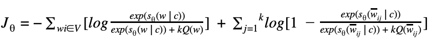
If we replace the final NCE equation with the equation above, we get:

Since log(1)=0,
therefore,

Since we’re dealing with sigmoid function i.e.

we can modify the equation above to:

(Here are the links to the Notebook and original paper)
Final thoughts and conclusion
We explored the evolution of neural-based modelling for NLP or machine translation. We covered word embedding, a method to find semantic, syntactic and linear relationship in the vocabulary. Although some of the methods mentioned earlier are no longer used, they lay the basic foundation of the subject, and make further learning easier.
We saw how Begio and his team introduced neural language models to find better representation through their word embedding method, followed by how Mikolov and his team modified Begio’s method and introduced a computationally less expensive method by removing the hidden layer. Although the word2vec model is a simple model, it became computationally expensive once the vocabulary size increased.
Different methods were introduced to rectify the issue of complexities, and the three models that we saw later in the post addressed the issue with the softmax function.
In the end, we saw how negative sampling outranks all the two methods (hierarchical softmax and NCE), and modifies word2vec model with a much more efficient approximation technique that captures better representation like semantic, syntactic, and preserves linear representation as well reduces the computational cost.
Word embedding opened new doors for NLP research and development. These models work well, but they still lack conceptual understanding. It was only in 2018 that Peters et. al. introduced ELMo: Embeddings from Language Model, which linked the missing piece of finding contextual representation through word embeddings.
For better understanding and clarity, check out the notebooks for each topic.
Resources
- On word embeddings – Part 1
- On word embeddings – Part 2: Approximating the Softmax
- Noise Contrastive Estimation
- The Illustrated Word2vec
- Distributed Representations of Words and Phrases and their Compositionality
- Efficient Estimation of Word Representations in Vector Space
- A Neural Probabilistic Language Model
- Notes on Noise Contrastive Estimation and Negative Sampling
