ARIMA & SARIMA: Real-World Time Series Forecasting

Time series and forecasting have been some of the key problems in statistics and Data Science. A data becomes a time series when it’s sampled on a time-bound attribute like days, months, and years inherently giving it an implicit order. Forecasting is when we take that data and predict future values. 

ARIMA and SARIMA are both algorithms for forecasting. ARIMA takes into account the past values (autoregressive, moving average) and predicts future values based on that. SARIMA similarly uses past values but also takes into account any seasonality patterns. Since SARIMA brings in seasonality as a parameter, it’s significantly more powerful than ARIMA in forecasting complex data spaces containing cycles.

May interest you

️ How to Select a Model For Your Time Series Prediction Task [Guide]

Further in the blog, we’re going to explore:

1. ARIMA
   • What it is and how it forecasts
   • Example of predicting GDP of USA using ARIMA
2. SARIMA
   • What it is and how it forecasts
   • Example of predicting electricity consumption
3. Pros and cons of both models
4. Real-world use-cases of ARIMA and SARIMA

Before we move on to the algorithms, there’s an important section about data processing that you should be wary about before embarking on your forecasting journey.

Data preprocessing for time series forecasting

Time series data is messy. Forecasting models from simple rolling averages to LSTMs requires data to be clean. So here are some techniques you could use before moving to forecasting.

Note: This data preprocessing step is general and intended to make readers emphasize it as real-world projects involve a lot of cleaning and preparation.

• Detrending/ Stationarity: Before forecasting, we want our time series variables to be mean-variance stationery. This means that the statistical properties of a model do not vary depending on when the sample was taken. Models built on stationary data are generally more robust. This can be achieved by using differencing.
• Anomaly detection: Any outlier present in the data might skew the forecasting results so it’s often considered a good practice to identify and normalize outliers before moving on to forecasting. You could follow this blog here where I have explained anomaly detection algorithms at length.
• Check for sampling frequency: This is an important step to check the regularity of sampling. Irregular data has to be imputed or made uniform before applying any modeling techniques because irregular sampling leads to broken integrity of the time series and doesn’t fit well with the models.
• Missing data: At times there can be missing data for some datetime values and it needs to be addressed before modeling. For example, a time series data with missing values looks like this:

Now, let’s move on to the models.

ARIMA 

ARIMA model is a class of linear models that utilizes historical values to forecast future values. ARIMA stands for Autoregressive Integrated Moving Average, each of which technique contributes to the final forecast. Let’s understand it one by one.

Autoregressive (AR)

In an autoregression model, we forecast the variable of interest using a linear combination of past values of that variable. The term autoregression indicates that it is a regression of the variable against itself. That is, we use lagged values of the target variable as our input variables to forecast values for the future. An autoregression model of order p will look like:

m_t = ₀ + ₁m_t-1 + ₂m_t-2 + ₃m_t-3+…+ _pm_t-p

In the above equation, the currently observed value of m is a linear function of its past p values. [ 0, p] are the regression coefficients that are determined after training. There are some standard methods to determine optimal values of p one of which is, analyzing Autocorrelation and Partial Autocorrelation function plots. 

The autocorrelation function (ACF) is the correlation between the current and the past values of the same variable. It also considers the translative effect that values carry over with time apart from a direct effect. For example, prices of oil 2 days ago will affect prices 1 day ago and eventually, today. But the prices of oil 2 days ago might also have an effect on today which ACF measures.

Partial Autocorrelation (PACF) on the other hand measures only the direct correlation between past values and current values. For example, PACF will only measure the effect of prices of oil 2 days ago on today with no translative effect.

ACF and PACF plots help us determine past value dependency which in turn helps us deduce p in AR. Head over here to understand how to deduce values for p (AR), and q(MA) in depth. 

Integrated (I)

Integrated represents any differencing that has to be applied in order to make the data stationary. A dickey-fuller test (code below) can be run on the data to check for stationarity and then experiment with different differencing factors. A differencing factor, d=1 means a lag of i.e.mt-mt-1. Let’s look at a plot of original vs differenced data.

The difference between them is evident. After differencing we could see that it’s significantly more stationary than the original and the mean and variance are approximately consistent over the years. We could use the code below to conduct a dickey-fuller test.

def check_stationarity(ts):
    dftest = adfuller(ts)
    adf = dftest[0]
    pvalue = dftest[1]
    critical_value = dftest[4]['5%']
    if (pvalue < 0.05) and (adf < critical_value):
        print('The series is stationary')
    else:
        print('The series is NOT stationary')

Moving Average (MA)

Moving average models uses past forecast errors rather than past values in a regression-like model to forecast future values. A moving average model can be denoted by the following equation:

m_t = ₀ + ₁e_t-1 + ₂e_t-2 + ₃e_t-3+…+ _qe_t-q

This is referred as MA(q) model. In the above equation, e is called an error and it represents the random residual deviations between the model and the target variable. Since e can only be determined after fitting the model and since it’s a parameter too so in this case e is an unobservable parameter. Hence, to solve the MA equation, iterative techniques like Maximum Likelihood Estimation are used instead of OLS.

Since we’ve looked at how ARIMA works, let’s dive into an example and see how ARIMA is applied to time series data.

Implementing ARIMA

For the implementation, I’ve chosen catfish sales data from 1996 to 2008. We’re going to apply the techniques we learned above to this dataset and see them in action. Although the data doesn’t need a lot of cleaning and is in a read-to-be-analyzed state, you might have to apply cleaning techniques to your dataset. 

Unfortunately, we cannot replicate each and every scenario as cleaning methods are highly subjective and depend on the team’s requirements too. But the techniques learned here can be directly applied to your dataset after cleaning.

Let’s start with importing essential modules.

Importing dependencies

from IPython.display import display

import numpy as np
import pandas as pd
pd.set_option('display.max_rows', 15)
pd.set_option('display.max_columns', 500)
pd.set_option('display.width', 1000)

import matplotlib.pyplot as plt
from datetime import datetime
from datetime import timedelta
from pandas.plotting import register_matplotlib_converters

register_matplotlib_converters()

from statsmodels.tsa.seasonal import seasonal_decompose
from statsmodels.tsa.arima_model import ARIMA
from statsmodels.tsa.statespace.sarimax import SARIMAX
from statsmodels.tsa.stattools import adfuller
from statsmodels.graphics.tsaplots import plot_acf, plot_pacf
from time import time
import seaborn as sns
sns.set(style="whitegrid")

import warnings
warnings.filterwarnings('ignore')

RANDOM_SEED = np.random.seed(0)

These are pretty self-explanatory modules every Data Scientist will be familiar with. It’s always a good practice to set the RANDOM_SEED to make code reproducible with the same results.

Next, we’re going to import and plot the time series data

Extract-Transform-Load (ETL)

def parser(s):
    return datetime.strptime(s, '%Y-%m-%d')
#read data
catfish_sales = pd.read_csv('catfish.csv', parse_dates=[0], index_col=0, date_parser=parser)
#infer the frequency of the data
catfish_sales = catfish_sales.asfreq(pd.infer_freq(catfish_sales.index))

#transform
start_date = datetime(1996,1,1)
end_date = datetime(2008,1,1)
lim_catfish_sales = catfish_sales[start_date:end_date]

#plot
plt.figure(figsize=(14,4))
plt.plot(lim_catfish_sales)
plt.title('Catfish Sales in 1000s of Pounds', fontsize=20)
plt.ylabel('Sales', fontsize=16)

For the sake of simplicity, I’ve limited the data to only 1996-2008. The plot generated by above code looks like:

First impressions say there is a definite trend and seasonality present in the data. Let’s do an STL decomposition to get a better understanding.

STL decomposition

plt.rc('figure',figsize=(14,8))
plt.rc('font',size=15)

result = seasonal_decompose(lim_catfish_sales,model='additive')
fig = result.plot()

Resulting plot look like this:

Points to ponder:

1. A 6-month and 12-month seasonal pattern is visible
2. An upwards and downwards trend is evident

Let’s look at ACF and PACF plots to get an idea for p and q values

ACF and PACF plots

plot_acf(lim_catfish_sales['Total'], lags=48);
plot_pacf(lim_catfish_sales['Total'], lags=30);

The output of the above code plots ACF and PACF:

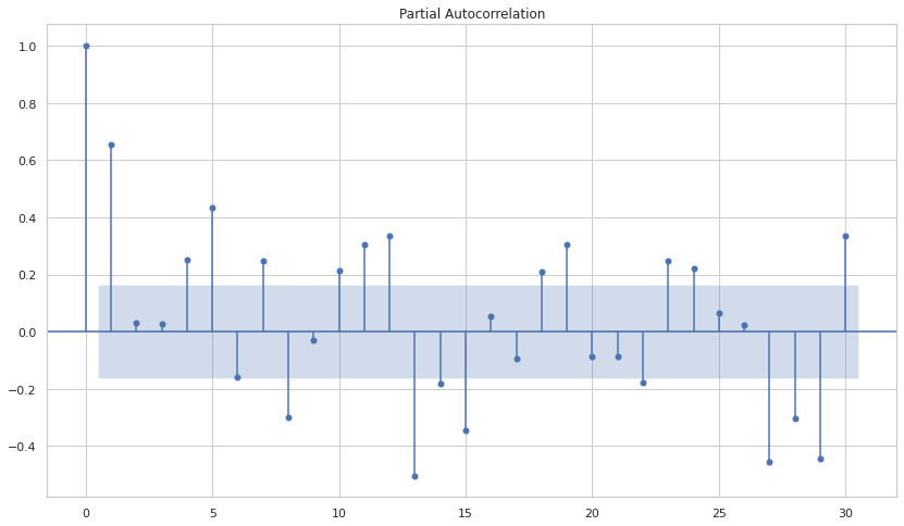
Points to ponder:

1. There’s a significant spike at 6-month and 12-month in ACF
2. PACF is nearly sinusoidal

The differencing factor d should be kept at 1 since there’s a clear trend and non-stationary data. P can be tested with values 6 and 12. 

Fitting ARIMA

We’re going to use statsmodels module to implement and use ARIMA. For this, we’ve imported the ARIMA class from the statsmodels. Now, let’s fit with the parameters we discussed in the previous section.

arima = ARIMA(lim_catfish_sales['Total'], order=(12,1,1))
predictions = arima.fit().predict()

As you notice above I started with (12,1,1) for (p,d,q) right from what we saw in the ACF and PACF plots. 

Note: It is quite handy to use modules for algorithms (like scikit-learn) and you’ll be glad to know that statsmodels is one of the libraries that gets used a lot.

Check more tools

Time Series Projects: Tools, Packages, and Libraries That Can Help

Let’s see how our predictions stack up with the original data.

Visualizing the result

plt.figure(figsize=(16,4))
plt.plot(lim_catfish_sales.diff(), label="Actual")
plt.plot(predictions, label="Predicted")
plt.title('Catfish Sales in 1000s of Pounds', fontsize=20)
plt.ylabel('Sales', fontsize=16)
plt.legend()

The output of the above code will give you a comparative plot of predictions and the actual data.

You can witness here that the model didn’t really catch up with some of the peaks but captured the essence of the data well. We can experiment with more p,d,q values to generalize the model better and make sure it doesn’t overfit.

Trial and optimization is one way but you can also use Auto-ARIMA. It essentially does the heavy lifting for you and tunes the hyperparameters for you. This blog is a good starting point for auto-ARIMA.

Keep in mind that the explainability of the parameters will be something that you have to deal with while working on Auto-ARIMA and make sure it doesn’t get converted into a BlackBox as forecasting models have to go for governance before deployment. So, it’s good practice to be able to explain the parameter values and their contribution.

SARIMA

SARIMA stands for Seasonal-ARIMA and it includes seasonality contribution to the forecast. The importance of seasonality is quite evident and ARIMA fails to encapsulate that information implicitly.

The Autoregressive (AR), Integrated (I), and Moving Average (MA) parts of the model remain as that of ARIMA. The addition of Seasonality adds robustness to the SARIMA model. It’s represented as:

where m is the number of observations per year. We use the uppercase notation for the seasonal parts of the model, and lowercase notation for the non-seasonal parts of the model. 

Similar to ARIMA, the P,D,Q values for seasonal parts of the model can be deduced from the ACF and PACF plots of the data. Let’s implement SARIMA for the same Catfish sales model.

Implementing SARIMA

The ETL and dependencies will remain the same as in ARIMA so we’ll jump straight to the modeling part.

Fitting SARIMA

sarima = SARIMAX(lim_catfish_sales['Total'],
                order=(1,1,1),
                seasonal_order=(1,1,0,12))
predictions = sarima.fit().predict()

I experimented with taking 1,1,1 for the non-seasonal parts and took 1,1,0,12 for seasonal ones as ACF showed a 6-month and 12-month lagged correlation. Let’s see how it turned out.

Visualizing the result

plt.figure(figsize=(16,4))
plt.plot(lim_catfish_sales, label="Actual")
plt.plot(predictions, label="Predicted")
plt.title('Catfish Sales in 1000s of Pounds', fontsize=20)
plt.ylabel('Sales', fontsize=16)
plt.legend()

As you can see, at the start model, struggled to fit probably because of off-course initialization but it quickly learned the right path. The fit is quite good as compared to the ARIMA one suggesting that SARIMA can learn seasonality better and if it’s present in the data then it’d make sense to try SARIMA out.

Pros and cons of ARIMA and SARIMA models

Owing to the linear nature of both the algorithms, they are quite handy and used in the industry when it comes to experimentation and understanding the data, creating baseline forecasting scores. If tuned right with lagged values (p,d,q) they can perform significantly better. The simple and explainable nature of both the algorithms makes them one of the top picks by analysts and Data Scientists. There are, however, some pros and cons when working with ARIMA and SARIMA at scale. Let’s discuss both of those:

Pros of ARIMA & SARIMA

• Easy to understand and interpret: The one thing that your fellow teammates and colleagues would appreciate is the simplicity and interpretability of the models. Focusing on both of these things while also maintaining the quality of the results will help with presentations with the stakeholders.
• Limited variables: There are fewer hyperparameters so the config file will be easily maintainable if the model goes into production.

Cons of ARIMA & SARIMA

• Exponential time complexity: When the value of p and q increases there are equally more coefficients to fit hence increasing the time complexity manifold if p and q are high. This makes both of these algorithms hard to put into production and makes Data Scientists look into Prophet and other algorithms. Then again, it depends on the complexity of the dataset too.
• Complex data: There can be a possibility where your data is too complex and there is no optimal solution for p and q. Although highly unlikely that ARIMA and SARIMA would fail but if this occurs then unfortunately you may have to look elsewhere.
• Amount of data needed: Both the algorithms require considerable data to work on, especially if the data is seasonal. For example, using three years of historical demand is likely not to be enough (Short Life-Cycle Products) for a good forecast.

May interest you

️ ARIMA vs Prophet vs LSTM for Time Series Prediction

Real-world use-cases of ARIMA and SARIMA

ARIMA/SARIMA are among the most popular econometrics models used for forecasting stock prices, demand forecasting, and even the spread of infectious diseases. When the underlying mechanisms are not known or are too complicated, e.g., the stock market, or not fully known, e.g., retail sales, it is usually better to apply ARIMA or a similar statistical model than complex deep algorithms like RNNs.

However, there are cases where applying ARIMA can give you par results. 

Here are some curated papers that use ARIMA/SARIMA:

1. An Application of ARIMA Model to Forecast the Dynamics of COVID-19 Epidemic in India: This research paper utilized ARIMA to forecast COVID-19 cases numbers in India. The shortcoming of utilizing ARIMA, in this case, is, that it only utilizes past values to forecast the future. But with COVID-19 changes shape with the passage of time and it depends on a lot of other behavioral factors other than past values that ARIMA isn’t capable to capture.
2. Time Series ARIMA Model for Prediction of Daily and Monthly Average Global Solar Radiation: The Case Study of Seoul, South Korea: This is a study that forecasts solar radiation in South Korea based on the hourly solar radiation data obtained from the Korean Meteorological Administration over 37 years by using SARIMA.
3. Disease management with ARIMA model in time series: Another example of using ARIMA in disease management utilizing wide applicability of ARIMA/SARIMA models. The research papers touch on some real-life use cases for ARIMA. For example, a hospital in Singapore accurately predicted the number of beds they will be needing in 3 days during the SARS epidemic.
4. Forecasting of demand using the ARIMA model: This use case focuses on modeling and forecasting demand in a food company using ARIMA.

When it comes to the industry, here’s a nice article about forecasting in Uber.

More often than not you’ll find ARIMA/SARIMA used when the problem statement is limited to the past values whether it’s predicting hospital beds, COVID cases, or forecasting demand. The shortcoming, however, arises when there are other factors to consider in forecasting like attributes that are static. Look out for the problem statement you’re working on, if these circumstances occur for you then try to use other methods like Theta, QRF (quantile regression forests), Prophet, RNNs. 

Conclusion and final notes

You’ve reached the end! In this blog, we discussed ARIMA and SARIMA at length pertaining to their utilization and importance for research in the industry. Their simplicity and robustness make them top contenders for modeling and forecasting. There are however some things to keep in mind while working on them in your real-world use case:

1. Increasing p,q can increase the time complexity of training exponentially. So, it’s advised to deduce their values priorly and then experiment.
2. They are prone to overfitting. So, make sure you set the hyperparameters right and do validation before moving to production.

That’s it from my side. Keep learning and stay tuned for more! Adios!

References

1. https://neptune.ai/blog/time-series-prediction-vs-machine-learning
2. https://otexts.com/fpp2/arima.html
3. https://towardsdatascience.com/understanding-arima-time-series-modeling-d99cd11be3f8
4. https://towardsdatascience.com/understanding-sarima-955fe217bc77
5. https://neptune.ai/blog/anomaly-detection-in-time-series
6. https://www.statsmodels.org/dev/generated/statsmodels.tsa.statespace.sarimax.SARIMAX.html
7. https://otexts.com/fpp2/seasonal-arima.html
8. https://towardsdatascience.com/time-series-forecasting-using-auto-arima-in-python-bb83e49210cd
9. https://towardsdatascience.com/time-series-from-scratch-autocorrelation-and-partial-autocorrelation-explained-1dd641e3076f
10. https://eng.uber.com/forecasting-introduction/
11. https://www.capitalone.com/tech/machine-learning/understanding-arima-models/
12. https://medium.com/analytics-vidhya/why-you-should-not-use-arima-to-forecast-demand-196cc8b8df3d