Neptune Blog

XGBoost: Everything You Need to Know

Aymane Hachcham

8 min

8th May, 2025

ML Tools

XGBoost is a popular gradient-boosting framework that supports GPU training, distributed computing, and parallelization. It’s precise, it adapts well to all types of data and supervised learning problems, it has excellent documentation, and overall, it’s very easy to use.

Over many years, it has become the de facto standard algorithm for getting accurate results from predictive modeling with machine learning. It’s one of the fastest gradient-boosting libraries for R, Python, and C++..

We are going to explore how to use XGBoost’s models and how to track their performance using Neptune. If you’re not sure that XGBoost is a great choice for you, follow along with the tutorial until the end, and then you’ll be able to make a fully informed decision.

What are ensemble algorithms?

Ensemble learning combines several learners (models) to improve overall performance, increasing predictiveness and accuracy in machine learning and predictive modeling.

Technically speaking, the power of ensemble models is simple: they can combine thousands of smaller learners trained on subsets of the original data. This can lead to interesting observations, like:

The variance of the general model decreases significantly thanks to bagging.
The bias also decreases due to boosting.
And overall predictive power improves because of stacking.

Types of ensemble methods

Ensemble methods can be classified into two groups based on how the sub-learners are generated:

Sequential ensemble methods: learners are generated sequentially. These methods use the dependency between base learners. A popular example of sequential ensemble algorithms is AdaBoost.

Parallel ensemble methods: learners are generated in parallel. The base learners are created independently to study and exploit the effects related to their independence and reduce error by averaging the results. An example of implementing this approach is Random Forests.

Ensemble methods can use homogeneous learners (learners from the same family) or heterogeneous learners (learners from multiple sorts, as accurate and diverse as possible).

Homogenous and heterogenous ML algorithms

Homogeneous ensemble methods typically use a single type of base learning algorithm, diversifying the training data by weighting samples.

Heterogeneous ensembles, on the other hand, consist of members with different base learning algorithms that can be combined and used simultaneously to form the predictive model.

A general rule of thumb:

Heterogeneous ensembles use different feature selection methods with the same data.
Homogeneous ensembles use the same feature selection with a variety of data and distribute the dataset over several nodes.

Homogeneous Ensembles:

Ensemble algorithms that use bagging, like Decision Tree Classifiers
Random Forests, Randomized Decision Trees

Heterogeneous Ensembles:

Support Vector Machines, SVM
Artificial Neural Networks, ANN
Memory-Based Learning methods
Bagged and Boosted decision Trees like XGBoost

Important characteristics of ensemble algorithms

Bagging

Bagging, short for Bootstrap Aggregating, is a technique that reduces overall variance by combining multiple models. It works by creating multiple subsets of the original dataset through random sampling with replacement, a process known as bootstrapping. A separate model is then trained on each of these subsets. When making predictions, bagging combines the outputs of all these models. For classification problems, such as in Random Forests, it typically uses majority voting to determine the final prediction. For regression problems, it usually averages the predictions of all models. This approach improves overall performance by mitigating the impact of individual model errors, effectively decreasing the variance of the final prediction.

Ensemble algorithms - begging — Bagging in Financial Machine Learning: Sequential Bootstrapping | Source

Note: Remember that some learners are stable and less sensitive to training perturbations. Such learners, when combined, don’t help the general model improve generalization performance.

Boosting

This technique matches weak learners—learners that have poor predictive power and do slightly better than random guessing—to a specific weighted subset of the original dataset. Higher weights are given to subsets that were misclassified earlier.

Learner predictions are then combined with voting mechanisms in the case of classification or a weighted sum for regression.

Ensemble algorithms - boosting — Intuition behind the boosting algorithm | Source

Well-known boosting algorithms

AdaBoost

AdaBoost stands for Adaptive Boosting. The logic implemented in the algorithm is:

First-round classifiers (learners) are all trained using equally weighted coefficients.
In subsequent boosting rounds, the adaptive process increasingly weighs data points that were misclassified by the learners in previous rounds and decreases the weights for correctly classified ones.

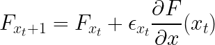
If you’re curious about the algorithm’s description, take a look at the image below:

Ensemble algorithms - adaboost — AdaBoost algo description in pseudocode | Source

Gradient Boosting

Gradient Boosting uses differentiable function losses from weak learners to generalize. At each boosting stage, the learners are used to minimize the loss function given the current model. Boosting algorithms can be used either for classification or regression.

What is XGBoost architecture?

XGBoost stands for eXtreme Gradient Boosting. It’s a parallelized and carefully optimized version of the gradient boosting algorithm. Parallelizing the whole boosting process improves the training time significantly.

Instead of training the best possible model on the data (like in traditional methods), we train thousands of models on various subsets of the training dataset and then vote for the best-performing model.

In many cases, XGBoost is better than usual gradient-boosting algorithms. The Python implementation gives access to a vast number of inner parameters to tweak for better precision and accuracy.

Some important features of XGBoost are:

Parallelization: The model is implemented to train with multiple CPU cores.
Regularization: XGBoost includes different regularization penalties to avoid overfitting. Penalty regularizations produce successful training, so the model can generalize adequately.
Non-linearity: XGBoost can detect and learn from non-linear data patterns.
Cross-validation: built-in and comes out-of-the-box.
Scalability: XGBoost can run distributedly thanks to distributed servers and clusters like Hadoop and Spark, so you can process enormous amounts of data. It’s also available in many programming languages like C++, JAVA, Python, and Julia.

For more details and an in-depth look at the mathematics behind gradient boosting, I recommend you check out this post by Krishna Kumar Mahto.

Other Gradient Boosting methods

Gradient Boosting Machine (GBM)

GBM combines predictions from multiple decision trees, and all the weak learners are decision trees. The key idea with this algorithm is that every node of those trees takes a different subset of features to select the best split. As it’s a Boosting algorithm, each new tree learns from the errors made in the previous ones.

Useful reference -> Understanding Gradient Boosting Machines

Light Gradient Boosting Machine (LightGBM)

LightGBM can handle huge amounts of data. It’s one of the fastest algorithms for both training and prediction. It generalizes well, meaning that it can be used to solve similar problems. It scales well to large numbers of cores and has open-source code, so you can use it in your projects for free.

Categorical Boosting (CatBoost)

The CatBoost algorithm, a specific form of gradient boosting, specializes in working with very diverse kinds of data. It shines with categorical data, but it also does well with numeric data and with datasets that contain both kinds of variables. Most gradient-boosting algorithms can work reasonably well with categorical variables, but CatBoost outperforms them because of how it handles these variables. Not only is CatBoost good at learning with the kinds of variables that many machine learning models struggle with, but it also learns efficiently from unlabeled data—that is, from data without any obvious outcomes or targets.

Integrating XGBoost with neptune.ai

Even though XGBoost is very powerful without hyperparameter tuning, you are likely to spend much of your time experimenting with different model architectures and feature engineering techniques for your given problem. After a few experiments, keeping track of the results of each run becomes nearly impossible due to the vast amount of metadata you have to record.

For this reason, XGBoost’s best friend is an experiment tracking library like Neptune. Neptune offers an XGBoost integration that can automatically capture all the training details and any additional metadata and visualize them nicely in a dashboard.

We will see how to use XGBoost in combination with Neptune on a regression problem using a sample dataset.

Disclaimer

Please note that this article references a deprecated version of Neptune.

For information on the latest version with improved features and functionality, please visit our website.

Setting up the environment

After signing up for an account, create your first Neptune project to store XGBoost models and their related metadata. Then, open up your terminal and create a virtual environment:

conda create -n neptune_xgboost python=3.9 -y
conda activate neptune_xgboost

Then, install the libraries we will need:

pip install neptune neptune-xgboost xgboost scikit-learn pandas seaborn ipykernel python-dotenv

Here is what the libraries do:

neptune.ai: Experiment tracking platform
neptune-xgboost: Neptune integration for XGBoost
xgboost: Gradient boosting library
scikit-learn: Machine learning tools and utilities
pandas: Data manipulation and analysis
seaborn: Statistical data visualization
ipykernel: IPython kernel for Jupyter
python-dotenv: Reading environment variables in Python

These libraries provide a comprehensive set of tools for data processing, model training, evaluation, visualization, and experiment tracking in a machine-learning workflow specifically tailored for XGBoost with Neptune integration.

If you are going to use Jupyter notebooks instead of Python scripts, run the following command to add the newly-created Conda environment as a Jupyter kernel:

ipython kernel install --user --name=neptune_xgboost

Next, create a file named .env in your current working directory:

touch .env

Paste the following contents into the file:

NEPTUNE_PROJECT_NAME="your/project-name"
NEPTUNE_API_TOKEN="your-neptune-api-token"

Now, you are ready to write some code!

Loading a sample dataset

We will use the Diamonds dataset, which is built into Seaborn:

import neptune
import xgboost as xgb
import seaborn as sns
import pandas as pd
from sklearn.model_selection import train_test_split

# Load and prepare data
diamonds = sns.load_dataset("diamonds")
diamonds.head()

As you can see, the dataset contains categorical features that need to be encoded. We will use the get_dummies() function of Pandas to take care of them:

X = pd.get_dummies(diamonds.drop("price", axis=1))
y = diamonds["price"]

X_train, X_test, y_train, y_test = train_test_split(
    X, y, test_size=0.2, random_state=42
)

After encoding, we extract the target column, the price of diamonds, into the y variable and split the data. Next, we will build DMatrix objects, which are specialized classes to represent datasets in the most efficient way for XGBoost:

# Create DMatrix objects
dtrain = xgb.DMatrix(X_train, label=y_train)
dtest = xgb.DMatrix(X_test, label=y_test)

We will pass these objects to XGBoost during training.

Creating a Neptune run object

The next step is connecting your notebook or script to Neptune. The way we will do this is by creating a Neptune run object:

import os
from dotenv import load_dotenv

load_dotenv()

project_name = os.getenv("NEPTUNE_PROJECT_NAME")
api_token = os.getenv("NEPTUNE_API_TOKEN")

run = neptune.init_run(project=project_name, api_token=api_token)

First, we import the os and load_dotenv modules to read the environment variables stored in your .env file. Then, we create the project_name and api_token variables using the .getenv() function.

This allows us to create a run object with the init_run() function, establishing a connection between our environment and Neptune.

We can already log some metadata using the run object. Let’s add model parameters:

params = {"max_depth": 6, "eta": 0.1, "objective": "reg:squarederror"}

# Log parameters
run["parameters"] = params

Once the above line executes, you can visit your project dashboard and see the parameters logged there.

Training a model in XGBoost and logging metadata to neptune.ai

Now, we are ready to train our first XGBoost model:

from neptune.integrations.xgboost import NeptuneCallback

num_rounds = 100

# Create callback
neptune_callback = NeptuneCallback(
    run=run, log_tree=[0, 1, 2]
)

# Train the model
model = xgb.train(
    params,
    dtrain,
    num_rounds,
    evals=[(dtrain, "train"), (dtest, "test")],
    callbacks=[neptune_callback],
)

We start by importing the NeptuneCallback class and then define the number of boosting rounds. Following that, we initialize the callback class by passing the run object.

Then, the training is as simple as calling the train() function of xgb with the following parameters:

params: The dictionary of XGBoost parameters we defined earlier
dtrain: The training data in DMatrix format
num_rounds: The number of boosting rounds (iterations)
evals: A list of tuples, each containing a dataset and its name for evaluation during training
callbacks: A list of callback functions, including our neptune_callback

The evals parameter allows us to monitor both training and test performance during the training process. The callbacks parameter, with our neptune_callback, ensures that Neptune logs metrics and other relevant information at each iteration, providing real-time insights into the model’s training progress.

Once the above snippet finishes execution, call:

run.stop()

indicating that our first experiment has ended. You should receive an output like below:

[neptune] [info   ] Shutting down background jobs, please wait a moment...
[neptune] [info   ] Done!
[neptune] [info   ] All 0 operations synced, thanks for waiting!
[neptune] [info   ] Explore the metadata in the Neptune app: https://app.neptune.ai/community/xgboost-tutorial/e/XGB-1/metadata

with a link to the experiment’s run page on your dashboard.

Inspecting and analyzing the experiment results

Clicking on the link and switching to the charts pane brings you to plots like below:

If you switch to the Images tab, you should see a feature importance plot as well:

The XGBRegressor generally classifies the order of importance of each feature used for the prediction. A benefit of using gradient boosting is that, after the boosted trees are constructed, it is relatively straightforward to retrieve importance scores for each attribute. This can be done by computing a feature importance graph and visualizing the similarity between each feature (feature-wise or attribute-wise) within the boosted trees.

We can see that diamond carat and depth are the principal factors in a diamond’s price.

Overview of some XGBoost hyperparameters

Let’s take a closer look and try to explain the XGBRegressor hyperparameters:

learning_rate: Used to control and adjust the weighting of the internal model estimators. The learning_rate should always be a small value to force long-term learning.
max_depth: Indicates the depth degree of the estimators (trees in this case). Manipulate this parameter carefully, because it will cause the model to overfit.
alpha: A specific type of penalty regularization (L1) to help avoid overfitting
num_estimators: The number of estimators the model will be built upon.
num_boost_round: The number of boosting stages. Although num_estimators and num_boost_round remain quite the same, you should keep in mind that the num_boost_round should be re-tuned each time you update a parameter.

Versioning your model

You can store multiple versions of your model in binary format in Neptune. Neptune automatically saves the current version of the model once the training is finished, so you can always get back and load previous model versions to compare.

Under the Training section, you’ll find all relevant metadata that’s been stored:

The Neptune platform also lets you cross-compare all your experiments in a seamless manner. Simply check the experiments you want, and a specific view will appear that shows all the required information.

You can share any Neptune experiment by just sending a link.

Note: Using the team plan, you can share all your work and projects with your teammates.

How to hyper-tune the XGBRegressor

The most efficient way of dealing with parameter tuning when time and resources are not an issue is to run a gigantic Grid Search on all the parameters and wait for the algorithm to output the optimal solution. It’s good to do so if you’re exploiting a small or intermediate dataset. But for bigger datasets, this approach can very quickly turn into a nightmare and consume too much time and too many resources.

Tips for hyper-tuning XGBoost when dealing with huge datasets

A well-known saying among data scientists goes like this: “You can make your model do wonders if your data has some signal, and if it doesn’t have a signal, it doesn’t.”.

The most straightforward approach I suggest when having vast amounts of training data is to try to manually research the features that have a significant predictive impact.

Firstly, try to reduce your features. 100 or 200 features is a lot; you should try to narrow the scope of feature selection. You could also rely on SelectKBest to select the top performers according to a specific criterion, in which each feature scores a K number of points and is chosen accordingly.
Bad performance can also be related to the quality assessment of your testing dataset. The test data might represent a completely different subset of data than your training data. Therefore, you should try doing cross-validation so that the R-squared value on the features is confident enough and sufficiently reliable.
Finally, if you see that your hyperparameter tuning still has minimal impact, try to switch to simpler regression methods like linear regression, Lasso, and Elastic Net, instead of sticking to XGBRegression.

Since the data for our example isn’t that big, we can choose to go for the first option. However, since the goal here is to expose the more reliable option for model tuning that you can leverage, we’ll go for this option without hesitation. Keep in mind that if you know which hyperparameters have more impact on the data, you’ll have a much smaller scope of work.

Grid search

Fortunately, XGBoost implements the scikit-learn API, so it’s very easy to use Grid Search and start rolling out the optimal results for the model based on the set of original hyperparameters.

Let’s create a range of values that each hyperparameter can take:

# Define the parameter grid
param_grid = {
    'max_depth': [3, 5, 7],
    'learning_rate': [0.01, 0.1, 0.3],
    'n_estimators': [100, 200, 300]
}

# Create an XGBoost regressor
xgb_model = xgb.XGBRegressor(random_state=42)

We also create an XGBRegressor object using the Scikit-learn API of XGBoost, which is a requirement.

Now, we import one new module and a function:

from sklearn.model_selection import train_test_split, GridSearchCV
from sklearn.metrics import mean_squared_error

Then, we reprepare our data:

# Prepare the data
X = pd.get_dummies(diamonds.drop('price', axis=1))
y = diamonds['price']

# Split the data
X_train, X_test, y_train, y_test = train_test_split(X, y, test_size=0.2, random_state=42)

And pass it to the GridSearchCV class:

# Set up GridSearchCV
grid_search = GridSearchCV(
    estimator=xgb_model,
    param_grid=param_grid,
    cv=3,
    n_jobs=-1,
    verbose=2
)

# Fit GridSearchCV
grid_search.fit(X_train, y_train)

The class will find the best set of parameters from our defined range based on the RMSE score of each parameter combination. Once the execution finishes, you can call best_params_ attribute of the grid_search object to see the best found parameters:

# Print the best parameters and score
print("Best parameters:", grid_search.best_params_)
print("Best cross-validation score:", grid_search.best_score_)

Output:

Best parameters: {'learning_rate': 0.1,'max_depth': 7, 'n_estimators': 200}
Best cross-validation score: 0.9804051121075948

XGBoost pros and cons

Advantages

Gradient Boosting comes with an easy-to-read and interpretable algorithm, making most of its predictions easy to handle.
Boosting is a resilient and robust method that prevents and curbs over-fitting quite easily.
XGBoost performs very well on medium, small, and structured datasets with not too many features.
It is a great approach because the majority of real-world problems involve classification and regression, two tasks where XGBoost is the reigning king.

Disadvantages

XGBoost does not perform so well on sparse and unstructured data.
A common thing often forgotten is that Gradient Boosting is very sensitive to outliers since every classifier is forced to fix the errors in the predecessor learners.
The overall method is hardly scalable. This is because the estimators base their correctness on previous predictors, hence the procedure involves a lot of struggle to streamline.

Conclusion

We’ve covered many aspects of Gradient Boosting, starting from a theoretical point of view to a more practical path. Now you can see how easy it is to add experiment tracking and model management to your XGBoost training and hyper-tuning with Neptune.

As always, I’ll leave you with some useful references below, so you can expand your pool of knowledge even more and improve your coding skills.

Stay tuned for more content!

Was the article useful?

More about XGBoost: Everything You Need to Know

Check out our product resources and related articles below:

Product resource

How Cradle Achieved Experiment Tracking and Data Security Goals With Self-Hosted Neptune