MLOps Blog

Understanding GAN Loss Functions

Harshit Dwivedi

4 min

29th August, 2023

ML Model Development

Ian Goodfellow introduced Generative Adversarial Networks (GAN) in 2014. It was one of the most beautiful, yet straightforward implementations of Neural Networks, and it involved two Neural Networks competing against each other. Yann LeCun, the founding father of Convolutional Neural Networks (CNNs), described GANs as “the most interesting idea in the last ten years in Machine Learning“.

In simple words, the idea behind GANs can be summarized like this:

Two Neural Networks are involved.
One of the networks, the Generator, starts off with a random data distribution and tries to replicate a particular type of distribution.
The other network, the Discriminator, through subsequent training, gets better at classifying a forged distribution from a real one.
Both of these networks play a min-max game where one is trying to outsmart the other.

Easy peasy lemon squeezy… but when you actually try to implement them, they often don’t learn the way you expect them to. One common reason is the overly simplistic loss function.

In this blog post, we will take a closer look at GANs and the different variations to their loss functions, so that we can get a better insight into how the GAN works while addressing the unexpected performance issues.

Standard GAN loss function (min-max GAN loss)

The standard GAN loss function, also known as the min-max loss, was first described in a 2014 paper by Ian Goodfellow et al., titled “Generative Adversarial Networks“.

The generator tries to minimize this function while the discriminator tries to maximize it. Looking at it as a min-max game, this formulation of the loss seemed effective.

In practice, it saturates for the generator, meaning that the generator quite frequently stops training if it doesn’t catch up with the discriminator.

The Standard GAN loss function can further be categorized into two parts: Discriminator loss and Generator loss.

Discriminator loss

While the discriminator is trained, it classifies both the real data and the fake data from the generator.

It penalizes itself for misclassifying a real instance as fake, or a fake instance (created by the generator) as real, by maximizing the below function.

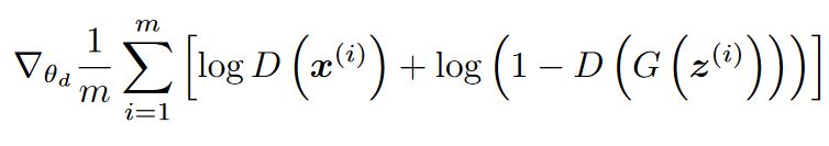
log(D(x)) refers to the probability that the generator is rightly classifying the real image,
maximizing log(1-D(G(z))) would help it to correctly label the fake image that comes from the generator.

Generator loss

While the generator is trained, it samples random noise and produces an output from that noise. The output then goes through the discriminator and gets classified as either “Real” or “Fake” based on the ability of the discriminator to tell one from the other.

The generator loss is then calculated from the discriminator’s classification – it gets rewarded if it successfully fools the discriminator, and gets penalized otherwise.

The following equation is minimized to training the generator:

Non-Saturating GAN Loss

A subtle variation of the standard loss function is used where the generator maximizes the log of the discriminator probabilities – log(D(G(z))).

This change is inspired by framing the problem from a different perspective, where the generator seeks to maximize the probability of images being real, instead of minimizing the probability of an image being fake.

This avoids generator saturation through a more stable weight update mechanism. In his blog, Daniel Takeshi compares the Non-Saturating GAN Loss along with some other variations.

Challenges with GAN loss functions

More often than not, GANs tend to show some inconsistencies in performance.

Most of these problems are associated with their training and are an active area of research.

Let’s look at some of them in detail:

Mode Collapse

This issue is on the unpredictable side of things. It wasn’t foreseen until someone noticed that the generator model could only generate one or a small subset of different outcomes or modes.

Usually, we would want our GAN to produce a range of outputs. We would expect, for example, another face for every random input to the face generator that we design.

Instead, through subsequent training, the network learns to model a particular distribution of data, which gives us a monotonous output which is illustrated below.

In the process of training, the generator is always trying to find the one output that seems most plausible to the discriminator.

Because of that, the discriminator’s best strategy is always to reject the output of the generator.

But if the next generation of discriminator gets stuck in a local minimum and doesn’t find its way out by getting its weights even more optimized, it’d get easy for the next generator iteration to find the most plausible output for the current discriminator.

This way, it will keep on repeating the same output and refrain from any further training.

Vanishing Gradients

This phenomenon happens when the discriminator performs significantly better than the generator. Either the updates to the discriminator are inaccurate, or they disappear.

One of the proposed reasons for this is that the generator gets heavily penalized, which leads to saturation in the value post-activation function, and the eventual gradient vanishing.

Convergence

Since there are two networks being trained at the same time, the problem of GAN convergence was one of the earliest, and quite possibly one of the most challenging problems since it was created.

The utopian situation where both networks stabilize and produce a consistent result is hard to achieve in most cases. One explanation for this problem is that as the generator gets better with next epochs, the discriminator performs worse because the discriminator can’t easily tell the difference between a real and a fake one.

If the generator succeeds all the time, the discriminator has a 50% accuracy, similar to that of flipping a coin. This poses a threat to the convergence of the GAN as a whole.

The image below shows this problem in particular:

As the discriminator’s feedback loses its meaning over subsequent epochs by giving outputs with equal probability, the generator may deteriorate its own quality if it continues to train on these junk training signals.

This medium article by Jonathan Hui takes a comprehensive look at all the aforementioned problems from a mathematical perspective.

Alternate GAN loss functions

Several different variations to the original GAN loss have been proposed since its inception. To a certain extent, they addressed the challenges we discussed earlier.

We will discuss some of the most popular ones which alleviated the issues, or are employed for a specific problem statement:

Wasserstein Generative Adversarial Network (WGAN)

This is one of the most powerful alternatives to the original GAN loss. It tackles the problem of Mode Collapse and Vanishing Gradient.

In this implementation, the activation of the output layer of the discriminator is changed from sigmoid to a linear one. This simple change influences the discriminator to give out a score instead of a probability associated with data distribution, so the output does not have to be in the range of 0 to 1.

Here, the discriminator is called critique instead, because it doesn’t actually classify the data strictly as real or fake, it simply gives them a rating.

Following loss functions are used to train the critique and the generator, respectively.

The output of the critique and the generator is not in probabilistic terms (between 0 and 1), so the absolute difference between critique and generator outputs is maximized while training the critique network.

Similarly, the absolute value of the generator function is maximized while training the generator network.

The original paper used RMSprop followed by clipping to prevent the weights values to explode:

Conditional Generative Adversarial Network (CGAN)

This version of GAN is used to learn a multimodal model. It basically generates descriptive labels which are the attributes associated with the particular image that was not part of the original training data.

CGANs are mainly employed in image labelling, where both the generator and the discriminator are fed with some extra information y which works as an auxiliary information, such as class labels from or data associated with different modalities.

The conditioning is usually done by feeding the information y into both the discriminator and the generator, as an additional input layer to it.

The following modified loss function plays the same min-max game as in the Standard GAN Loss function. The only difference between them is that a conditional probability is used for both the generator and the discriminator, instead of the regular one.

Why conditional probability? Because we are feeding in some auxiliary information(the green points), which helps in making it a multimodal model, as shown in the diagram below:

This medium article by Jonathan Hui delves deeper into CGANs and discusses the mathematics behind it.

Summary

In this blog, we discussed:

The original Generative Adversarial Networks loss functions along with the modified ones.
Different challenges of employing them in real-life scenarios.
Alternatives loss functions like WGAN and C-GAN.

The main goal of this article was to provide an overall intuition behind the development of the Generative Adversarial Networks. Hopefully, it gave you a better feel for GANs, along with a few helpful insights. Thanks for reading!