

Source: Supercharge your Computer Vision models with the TensorFlow Object Detection API,
Jonathan Huang, Research Scientist and Vivek Rathod, Software Engineer,
Google AI Blog
Object Detection as a task in Computer Vision
We encounter objects every day in our life. Look around, and you’ll find multiple objects surrounding you. As a human being you can easily detect and identify each object that you see. It’s natural and doesn’t take much effort.
For computers, however, detecting objects is a task that needs a complex solution. For a computer to “detect objects” means to process an input image (or a single frame from a video) and respond with information about objects on the image and their position. In computer vision terms, we call these two tasks classification and localization. We want the computer to say what kind of objects are presented on a given image and where exactly they’re located.
Multiple solutions have been developed to help computers detect objects. Today, we’re going to explore a state-of-the-art algorithm called YOLO, which achieves high accuracy at real-time speed. In particular, we’ll learn how to train this algorithm on a custom dataset in TensorFlow / Keras.
First, let’s see what exactly YOLO is and what it’s famous for.
YOLO as a real-time object detector
What is YOLO?
YOLO is an acronym for “You Only Look Once” (don’t confuse it with You Only Live Once from The Simpsons). As the name suggests, a single “look” is enough to find all objects on an image and identify them.
In machine learning terms, we can say that all objects are detected via a single algorithm run. It’s done by dividing an image into a grid and predicting bounding boxes and class probabilities for each cell in a grid. In case we’d like to employ YOLO for car detection, here’s what the grid and the predicted bounding boxes might look like:

Bounding box that YOLO predicts for the first car is in red.
Bounding box that YOLO predicts for the second car is yellow.
Source of the image.
The above image contains only the final set of boxes obtained after filtering. It’s worth noting that YOLO’s raw output contains many bounding boxes for the same object. These boxes differ in shape and size. As you can see in the image below, some boxes are better at capturing the target object whereas others offered by an algorithm perform poorly.

All yellow boxes are for the second car.
The bold red and yellow boxes are the best for car detection.
Source of the image.
To select the best bounding box for a given object, a Non-maximum suppression (NMS) algorithm is applied.

boxes predicted for the cars to keep only those that best capture objects.
Source of the image.
All boxes that YOLO predicts have a confidence level associated with them. NMS uses these confidence values to remove the boxes which were predicted with low certainty. Usually, these are all boxes that are predicted with confidence below 0.5.
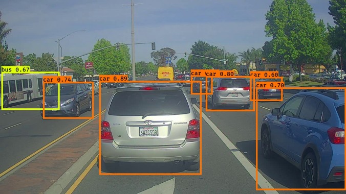
You can see the confidence scores in the top-left corner of each box, next to the object name.
Source of the image.
When all uncertain bounding boxes are removed, only the boxes with the high confidence level are left. To select the best one among the top-performing candidates, NMS selects the box with the highest confidence level and calculates how it intersects with the other boxes around. If an intersection is higher than a particular threshold level, the bounding box with lower confidence is removed. In case NMS compares two boxes that have an intersection below a selected threshold, both boxes are kept in final predictions.
YOLO compared to other detectors
Although a convolutional neural net (CNN) is used under the hood of YOLO, it’s still able to detect objects with real-time performance. It’s possible thanks to YOLO’s ability to do the predictions simultaneously in a single-stage approach.
Other, slower algorithms for object detection (like Faster R-CNN) typically use a two-stage approach:
- in the first stage, interesting image regions are selected. These are the parts of an image that might contain any objects;
- in the second stage, each of these regions is classified using a convolutional neural net.
Usually, there are many regions on an image with the objects. All of these regions are sent to classification. Classification is a time-consuming operation, which is why the two-stage object detection approach performs slower compared to one-stage detection.
YOLO doesn’t select the interesting parts of an image, there’s no need for that. Instead, it predicts bounding boxes and classes for the whole image in a single forward net pass.
Below you can see how fast YOLO is compared to other popular detectors.

SSD and YOLO are one stage object detectors whereas Faster-RCNN
and R-FCN are two-stage object detectors.
Source of the image.
Versions of YOLO
YOLO was first introduced in 2015 by Joseph Redmon in his research paper titled “You Only Look Once: Unified, Real-Time Object Detection”.
Since then, YOLO has evolved a lot. In 2016 Joseph Redmon described the second YOLO version in “YOLO9000: Better, Faster, Stronger”.
About two years after the second YOLO update, Joseph came up with another net upgrade. His paper, called “YOLOv3: An Incremental Improvement”, caught the attention of many computer engineers and became popular in the machine learning community.
In 2020, Joseph Redmon decided to stop researching computer vision, but it didn’t stop YOLO from being developed by others. That same year, a team of three engineers (Alexey Bochkovskiy, Chien-Yao Wang, Hong-Yuan Mark Liao) designed the fourth version of YOLO, even faster and more accurate than before. Their findings are described in the “YOLOv4: Optimal Speed and Accuracy of Object Detection” paper they published on April 23rd, 2020.
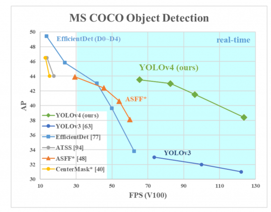
AP on the Y-axis is a metric called “average precision”. It describes the accuracy of the net.
FPS (frames per second) on the X-axis is a metric that describes speed.
Source of the image.
Two months after the release of the 4th version, an independent developer, Glenn Jocher, announced the 5th version of YOLO. This time, there was no research paper published. The net became available on Jocher’s GitHub page as a PyTorch implementation. The fifth version had pretty much the same accuracy as the fourth version but it was faster.
Lastly, in July 2020 we got another big YOLO update. In a paper titled “PP-YOLO: An Effective and Efficient Implementation of Object Detector”, Xiang Long and team came up with a new version of YOLO. This iteration of YOLO was based on the 3rd model version and exceeded the performance of YOLO v4.

The mAP on the Y-axis is a metric called “ mean average precision”. It describes the accuracy of the net.
FPS (frames per second) on the X-axis is a metric that describes speed.
Source of the image.
In this tutorial, we’re going to have a closer look at YOLOv4 and its implementation. Why YOLOv4? Three reasons:
- It has wide approval in the machine learning community;
- This version has proven its high performance in a broad range of detection tasks;
- YOLOv4 has been implemented in multiple popular frameworks, including TensorFlow and Keras, which we’re going to work with.
Examples of YOLO applications
Before we move on to the practical part of this article, implementing our custom YOLO based object detector, I’d like to show you a couple of cool YOLOv4 implementations, and then we’re going to make our implementation.
Pay attention to how fast and accurate the predictions are!
Here’s the first impressive example of what YOLOv4 can do, detecting multiple objects from different game and movie scenes.
Alternatively, you can check this object detection demo from a real-life camera view.
YOLO as an object detector in TensorFlow & Keras
TensorFlow & Keras frameworks in Machine Learning
Source of the image.
Frameworks are essential in every information technology domain. Machine learning is no exception. There are several established players in the ML market which help us simplify the overall programming experience. PyTorch, scikit-learn, TensorFlow, Keras, MXNet and Caffe are just a few worth mentioning.
Related posts
Today, we’re going to work closely with TensorFlow/Keras. Not surprisingly, these two are among the most popular frameworks in the machine learning universe. It’s largely due to the fact that both TensorFlow and Keras provide rich capabilities for development. These two frameworks are quite similar to each other. Without digging too much into details, the key thing to remember is that Keras is just a wrapper for the TensorFlow framework.
YOLO implementation in TensorFlow & Keras
At the time of writing this article, there were 808 repositories with YOLO implementations on a TensorFlow / Keras backend. YOLO version 4 is what we’re going to implement. Limiting the search to only YOLO v4, I got 55 repositories.
Carefully browsing all of them, I found an interesting candidate to continue with.
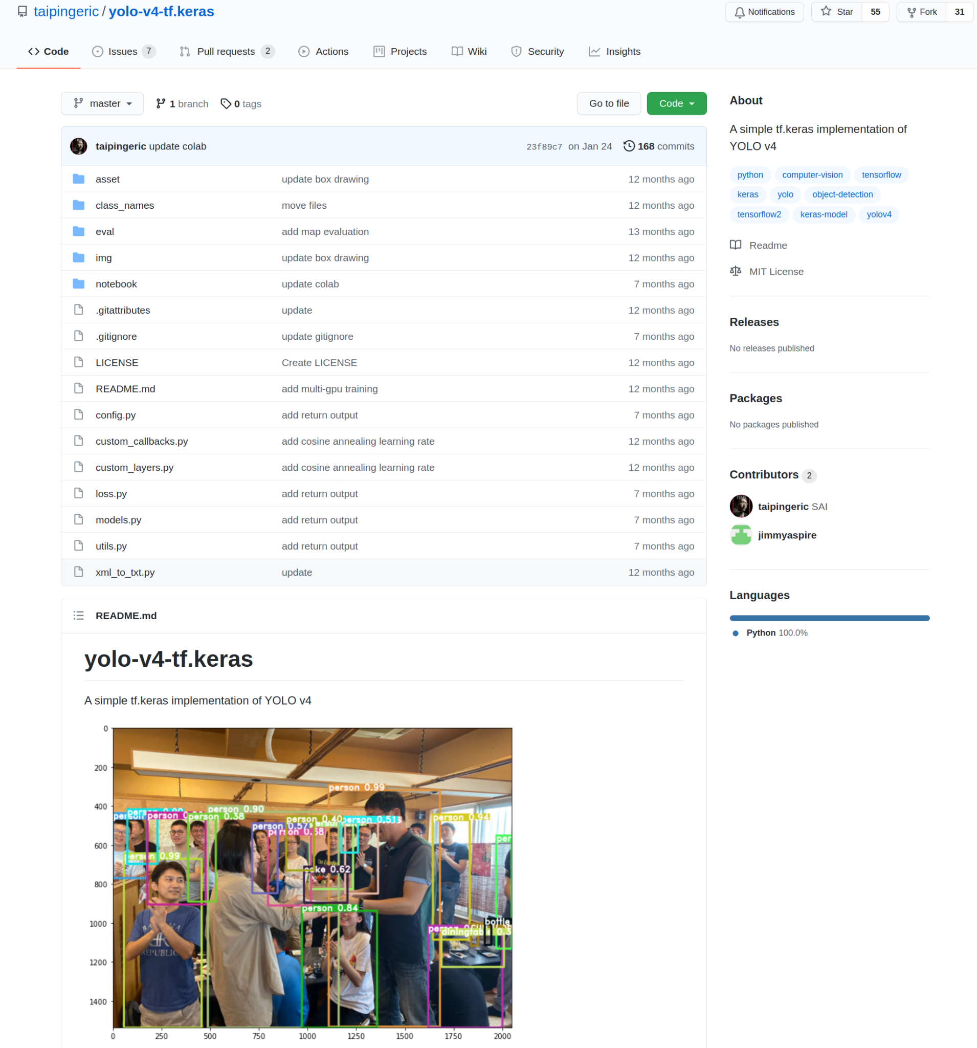
Source of the image.
This implementation was developed by taipingeric and jimmyaspire. It’s quite simple and very intuitive if you’ve worked with TensorFlow and Keras before.
To start working with this implementation, just clone the repo to your local machine. Next, I will show you how to use YOLO out of the box, and how to train your own custom object detector.
How to run pre-trained YOLO out-of-the-box and get results
Looking at the “Quick Start” section of the repo, you can see that to get a model up and running, we just have to import YOLO as a class object and load in the model weights:
from models import Yolov4
model = Yolov4(weight_path='yolov4.weights',
               class_name_path='class_names/coco_classes.txt')
Note that you need to manually download model weights in advance. The model weights file that comes with YOLO comes from the COCO dataset, and it’s available at the AlexeyAB official darknet project page at GitHub.
Right after, the model is fully ready to work with images in inference mode. Just use the predict() method for an image of your choice. The method is standard for TensorFlow and Keras frameworks.
pred = model.predict('input.jpg')
For example for this input image:

I got the following model output:

Predictions that the model made are returned in a convenient form of a pandas DataFrame. We get class name, box size, and coordinates for each detected object:

Lots of useful information about the detected objects
There are multiple parameters within the predict() method that let us specify whether we want to plot the image with the predicted bounding boxes, textual names for each object, etc. Check out the docstring that goes along with the predict() method to get familiar with what’s available to us:

You should expect that your model will only be able to detect object types that are strictly limited to the COCO dataset. To know what object types a pre-trained YOLO model is able to detect, check out the coco_classes.txt file available in …/yolo-v4-tf.kers/class_names/. There are 80 object types in there.
How to train your custom YOLO object detection model
Task statement

To design an object detection model, you need to know what object types you want to detect. This should be a limited number of object types that you want to create your detector for. It’s good to have a list of object types prepared as we move to the actual model development.
Ideally, you should also have an annotated dataset that has objects of your interest. This dataset will be used to train a detector and validate it. If you don’t yet have either a dataset or annotation for it, don’t worry, I’ll show you where and how you can get it.
Dataset & annotations
Where to get data from
If you have an annotated dataset to work with, just skip this part and move on to the next chapter. But, if you need a dataset for your project, we’re now going to explore online resources where you can get data.
It doesn’t really matter what field you’re working in, there’s a big chance that there’s already an open-source dataset that you can use for your project.
The first resource I recommend is the “50+ Object Detection Datasets from different industry domains” article by Abhishek Annamraju who has collected wonderful annotated datasets for industries such as Fashion, Retail, Sports, Medicine and many more.

Source of the image.
Other two great places to look for the data are paperswithcode.com and roboflow.com which provide access to high-quality datasets for object detection.
Check out these above assets to collect the data you need or to enrich the dataset that you already have.
How to annotate data for YOLO
If your dataset of images comes without annotations, you must do the annotation job yourself. This manual operation is quite time-consuming, so make sure you have enough time to do it.
As an annotation tool you might consider multiple options. Personally, I would recommend using LabelImg. It’s a light-weight and easy-to-use image annotation tool that can directly output annotations for YOLO models.
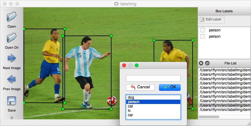
Source of the image.
How to transform data from other formats to YOLO
Annotations for YOLO are in the form of txt files. Each line in a txt file fol YOLO must have the following format:
image1.jpg 10,15,345,284,0
image2.jpg 100,94,613,814,0 31,420,220,540,1
We can break up each line from the txt file and see what it consists of:
- The first part of a line specifies the basenames for the images: image1.jpg, image2.jpg
- The second part of a line defines the bounding box coordinates and the class label. For example, 10,15,345,284,0 states for xmin,ymin,xmax,ymax,class_id
- If a given image has more than one object on it, there will be multiple boxes and class labels next to the image basename, divided by a space.
Bounding box coordinates are a clear concept, but what about the class_id number that specifies the class label? Each class_id is linked with a particular class in another txt file. For example, pre-trained YOLO comes with the coco_classes.txt file which looks like this:
person
bicycle
car
motorbike
aeroplane
bus
...
Number of lines in the classes files must match the number of classes that your detector is going to detect. Numeration starts from zero, meaning that the class_id number for the first class in the classes file is going to be 0. Class that is placed on the second line in the classes txt file will have number 1.
Now you know how the annotation for YOLO looks like. To continue creating a custom object detector I urge you to do two things now:
- create a classes txt file where you will palace of the classes that you want your detector to detect. Remember that class order matters.
- Create a txt file with annotations. In case you already have annotation but in the VOC format (.XMLs), you can use this file to transform from XML to YOLO.
Splitting data into subsets
As always, we want to split the dataset into 2 subsets: for training and for validation. It can be done as simple as:
from utils import read_annotation_lines

train_lines, val_lines = read_annotation_lines('../path2annotations/annot.txt', test_size=0.1)
Creating data generators
When the data is split, we can proceed to the data generator initialization. We’ll have a data generator for each data file. In our case, we’ll have a generator for the training subset and for the validation subset.
Here’s how the data generators are created:
from utils import DataGenerator

FOLDER_PATH = '../dataset/img'
class_name_path = '../class_names/bccd_classes.txt'

data_gen_train = DataGenerator(train_lines, class_name_path, FOLDER_PATH)
data_gen_val = DataGenerator(val_lines, class_name_path, FOLDER_PATH)
To sum everything up, here’s what the complete code for data splitting and generator creation looks like:
from utils import read_annotation_lines, DataGenerator

train_lines, val_lines = read_annotation_lines('../path2annotations/annot.txt', test_size=0.1)

FOLDER_PATH = '../dataset/img'
class_name_path = '../class_names/bccd_classes.txt'

data_gen_train = DataGenerator(train_lines, class_name_path, FOLDER_PATH)
data_gen_val = DataGenerator(val_lines, class_name_path, FOLDER_PATH)
Installation & setup required for model training
Let’s talk about the prerequisites that are essential to create your own object detector:
- You should have Python already installed on your computer. In case you need to install it, I recommend following this official guide by Anaconda;
- If your computer has a CUDA-enabled GPU (a GPU made by NVIDIA), then a few relevant libraries are needed in order to support GPU-based training. In case you need to enable GPU support, check the guidelines on NVIDIA’s website. Your goal is to install the latest version of both the CUDA Toolkit, and cuDNN for your operating system;
- You might want to organise an independent virtual environment to work in. This project requires TensorFlow 2 installed. All other libraries will be introduced later on;
- As for me, I was building and training my YOLOv4 model in a Jupyter Notebook development environment. Although Jupyter Notebook seems like a reasonable option to go with, consider development in an IDE of your choice if you wish.
Model training

Prerequisites
By now you should have:
- A split for your dataset;
- Two data generators initialized;
- A txt file with the classes.
Model object initialization
To get ready for a training job, initialize the YOLOv4 model object. Make sure that you use None as a value for the weight_path parameter. You also should provide a path to your classes txt file at this step. Here’s the initialization code that I used in my project:
class_name_path = 'path2project_folder/model_data/scans_file.txt'

model = Yolov4(weight_path=None,
               class_name_path=class_name_path)
The above model initialization leads to creation of a model object with a default set of parameters. Consider changing the configuration of your model by passing in a dictionary as a value to the config model parameter.

Config specifies a set of parameters for the YOLOv4 model.
Default model configuration is a good starting point but you may want to experiment with other configs for better model quality.
In particular, I highly recommend experimenting with anchors and img_size. Anchors specify the geometry of the anchors that will be used to capture objects. The better the shapes of the anchors fit the objects shapes, the higher the model performance will be.
Increasing img_size might be useful in some cases, too. Keep in mind that the higher the image is, the longer the model will do the inference.
In case you’d like to use neptune.ai as a tracking tool, you should also initialize an experiment run, like this:
import neptune

run = neptune.init_run(project="projects/my_project",
                   api_token=my_token)
Defining callbacks
TensorFlow & Keras let us use callbacks to monitor the training progress, make checkpoints, and manage training parameters (e.g. learning rate).
Before fitting your model, define callbacks that will be useful for your purposes. Make sure to specify paths to store model checkpoints and associated logs. Here’s how I did it in one of my projects:
 # defining pathes and callbacks

dir4saving = 'path2checkpoint/checkpoints'
os.makedirs(dir4saving, exist_ok = True)

logdir = 'path4logdir/logs'
os.makedirs(logdir, exist_ok = True)

name4saving = 'epoch_{epoch:02d}-val_loss-{val_loss:.4f}.hdf5'

filepath = os.path.join(dir4saving, name4saving)

rLrCallBack = keras.callbacks.ReduceLROnPlateau(monitor = 'val_loss',
                                             factor = 0.1,
                                             patience = 5,
                                             verbose = 1)

tbCallBack = keras.callbacks.TensorBoard(log_dir = logdir,
                                         histogram_freq = 0,
                                         write_graph = False,
                                         write_images = False)

mcCallBack_loss = keras.callbacks.ModelCheckpoint(filepath,
                                            monitor = 'val_loss',
                                            verbose = 1,
                                            save_best_only = True,
                                            save_weights_only = False,
                                            mode = 'auto',
                                            period = 1)

esCallBack = keras.callbacks.EarlyStopping(monitor = 'val_loss',
                                          mode = 'min',
                                          verbose = 1,
                                          patience = 10)
You could have noticed that in the above callbacks set TensorBoard is used as a tracking tool. Consider using Neptune as a much more advanced tool for experiment tracking. If so, don’t forget to initialize another callback to enable integration with Neptune:
from neptune.integrations.tensorflow_keras import NeptuneCallback

neptune_callback = NeptuneCallback(run=run, base_namespace="metrics")
Fitting the model
To kick off the training job, simply fit the model object using the standard fit() method in TensorFlow / Keras. Here’s how I started training my model:
model.fit(data_gen_train,
          initial_epoch=0,
          epochs=10000,
          val_data_gen=data_gen_val,
          callbacks=[rLrCallBack,
                     tbCallBack,
                     mcCallBack_loss,
                     esCallBack,
                     neptune_callback]
         )
When the training is started, you will see a standard progress bar.

The training process will evaluate the model at the end of every epoch. If you use a set of callbacks similar to what I initialized and passed in while fitting, those checkpoints that show model improvement in terms of lower loss will be saved to a specified directory.
If no errors occur and the training process goes smoothly, the training job will be stopped either because of the end of the training epochs number, or if the early stopping callback detects no further model improvement and stops the overall process.
In any case, you should end up with multiple model checkpoints. We want to select the best one from all available ones and use it for inference.
Trained custom model in inference mode
Running a trained model in the inference mode is similar to running a pre-trained model out of the box.

You initialize a model object passing in the path to the best checkpoint as well as the path to the txt file with the classes. Here’s what model initialization looks like for my project:
from models import Yolov4
model = Yolov4(weight_path='path2checkpoint/checkpoints/epoch_48-val_loss-0.061.hdf5',
               class_name_path='path2classes_file/my_yolo_classes.txt')
When the model is initialized, simply use the predict() method for an image of your choice to get the predictions. As a recap, detections that the model made are returned in a convenient form of a pandas DataFrame. We get the class name, box size, and coordinates for each detected object.
Conclusions
You’ve just learned how to create a custom YOLOv4 object detector. We’ve gone over the end-to-end process, starting from data collection, annotation, and transformation. You have enough knowledge about the fourth YOLO version and how it differs from other detectors.
Nothing stops you now from training your own model in TensorFlow and Keras. You know where to get a pre-trained model from and how to kick off the training job.
In my upcoming article, I will show you some of the best practices and life hacks that will help improve the quality of the final model. Stay with us!

