MLOps Blog

How to Use Google Colab for Deep Learning – Complete Tutorial

Harshit Dwivedi

8 min

14th November, 2023

ML Model Development ML Tools

If you’re a programmer, you want to explore deep learning, and need a platform to help you do it – this tutorial is exactly for you.

Google Colab is a great platform for deep learning enthusiasts, and it can also be used to test basic machine learning models, gain experience, and develop an intuition about deep learning aspects such as hyperparameter tuning, preprocessing data, model complexity, overfitting and more.

Let’s explore!

Introduction

Colaboratory by Google (Google Colab in short) is a Jupyter notebook based runtime environment which allows you to run code entirely on the cloud.

This is necessary because it means that you can train large scale ML and DL models even if you don’t have access to a powerful machine or a high speed internet access.

Google Colab supports both GPU and TPU instances, which makes it a perfect tool for deep learning and data analytics enthusiasts because of computational limitations on local machines.

Since a Colab notebook can be accessed remotely from any machine through a browser, it’s well suited for commercial purposes as well.

In this tutorial you will learn:

Getting around in Google Colab
Installing python libraries in Colab
Downloading large datasets in Colab
Training a Deep learning model in Colab
Using TensorBoard in Colab

LEARN MORE

How to Deal with Files in Google Colab: Everything You Need to Know

Creating your first .ipynb notebook in colab

Open a browser of your choice and go to colab.research.google.com and sign in using your Google account. Click on a new notebook to create a new runtime instance.

In the top left corner, you can change the name of the notebook from “Untitled.ipynb“ to the name of your choice by clicking on it.

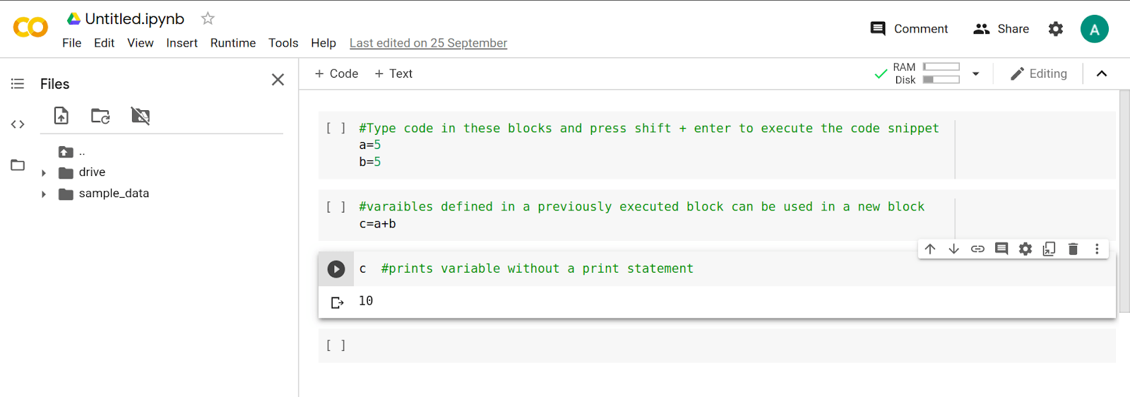
The cell execution block is where you type your code. To execute the cell, press shift + enter.

The variable declared in one cell can be used in other cells as a global variable. The environment automatically prints the value of the variable in the last line of the code block if stated explicitly.

Training a sample tensorflow model

Training a machine learning model in Colab is very easy. The best part about it is not having to set up a custom runtime environment, it’s all handled for you.

Setup:

#import necessary libraries
import tensorflow as tf

#load training data and split into train and test sets
mnist = tf.keras.datasets.mnist

(x_train,y_train), (x_test,y_test) = mnist.load_data()
x_train, x_test = x_train / 255.0, x_test / 255.0

The output for this code snippet will look like this:

Downloading data from https://storage.googleapis.com/tensorflow/tf-keras-datasets/mnist.npz
11493376/11490434 [==============================] - 0s 0us/step

Next, we define the Google Colab model using Python:

#define model
model = tf.keras.models.Sequential([
                               tf.keras.layers.Flatten(input_shape=(28,28)),
                                   tf.keras.layers.Dense(128,activation='relu'),
                                   tf.keras.layers.Dropout(0.2),
                                   tf.keras.layers.Dense(10)
])

#define loss function variable
loss_fn = tf.keras.losses.SparseCategoricalCrossentropy(from_logits=True)

#define optimizer,loss function and evaluation metric
model.compile(optimizer='adam',
             loss=loss_fn,
             metrics=['accuracy'])

#train the model
model.fit(x_train,y_train,epochs=5)

The expected output upon execution of the above code snippet is:

Epoch 1/5
1875/1875 [==============================] - 3s 2ms/step - loss: 0.3006 - accuracy: 0.9125
Epoch 2/5
1875/1875 [==============================] - 3s 2ms/step - loss: 0.1461 - accuracy: 0.9570
Epoch 3/5
1875/1875 [==============================] - 3s 2ms/step - loss: 0.1098 - accuracy: 0.9673
Epoch 4/5
1875/1875 [==============================] - 3s 2ms/step - loss: 0.0887 - accuracy: 0.9729
Epoch 5/5
1875/1875 [==============================] - 3s 2ms/step - loss: 0.0763 - accuracy: 0.9754
<tensorflow.python.keras.callbacks.History at 0x7f2abd968fd0>

#test model accuracy on test set
model.evaluate(x_test,y_test,verbose=2)

Expected output:

313/313 - 0s - loss: 0.0786 - accuracy: 0.9761
[0.07860152423381805, 0.9761000275611877]

#extend the base model to predict softmax output
probability_model = tf.keras.Sequential([
                                        model,
                                        tf.keras.layers.Softmax()])

Installing packages in Google Colab

You can use the code cell in Colab not only to run Python code but also to run shell commands. Just add a ! before a command. The exclamation point tells the notebook cell to run the following command as a shell command.

Most general packages needed for deep learning come pre-installed. In some cases, you might need less popular libraries, or you might need to run code on a different version of a library. To do this, you’ll need to install packages manually.

The package manager used for installing packages is pip.

To install a particular version of TensorFlow use this command:

!pip3 install tensorflow==1.5.0

The following output is expected after running the above command:

Click on RESTART RUNTIME for the newly installed version to be used.

As you can see above, we changed the Tensorflow version from ‘2.3.0’ to ‘1.5.0’.

The test accuracy is around 97% for the model we trained above. Not bad at all, but this was an easy one.

Training models usually isn’t that easy, and we often have to download datasets from third-party sources like Kaggle.

So let’s see how to download datasets when we don’t have a direct link available for us.

Downloading a dataset

When you’re training a machine learning model on your local machine, you’re likely to have trouble with the storage and bandwidth costs that come with downloading and storing the dataset required for training a model.

Deep learning datasets can be massive in size, ranging between 20 to 50 Gb. Downloading them is most challenging if you’re living in a developing country, where getting high-speed internet isn’t possible.

The most efficient way to use datasets is to use a cloud interface to download them, rather than manually uploading the dataset from a local machine.

Thankfully, Colab gives us a variety of ways to download the dataset from common data hosting platforms.

Downloading the dataset from Kaggle

To download an existing dataset from Kaggle, we can follow the steps outlined below:

Go to your Kaggle Account and click on “Create New API Token”. This will download a kaggle.json file to your machine.
Go to your Google Colab project file, and run the following commands:

! pip install -q kaggle
from google.colab import files

# choose the kaggle.json file that you downloaded
files.upload()
! mkdir ~/.kaggle

# make a directory named kaggle and copy the kaggle.json file there
cp kaggle.json ~/.kaggle/

# change the permissions of the file
! chmod 600 ~/.kaggle/kaggle.json

# download the dataset for a specific competition
! kaggle competitions download -c 'name-of-competition'

Downloading the dataset from any generic website

Depending on the browser that you’re using, there are extensions available to convert the dataset download link into `curl` or `wget` format. You can use this to efficiently download the dataset.

For Firefox, there’s the cliget browser extension: cliget – Get this Extension for Firefox (en-US)
For Chrome, there’s the CurlWget extension: Ad Added CurlWget 52

These extensions will generate a curl/wget command as soon as you click on any download button in your browser.

You can then copy that command and execute it in your Colab notebook to download the dataset.

NOTE: By default, the Colab notebook uses Python shell. To run terminal commands in Colab, you will have to use “!” at the beginning of the command.

For example, to download a file from some.url and save it as some.file, you can use the following command in Colab:

!curl http://some.url --output some.file

NOTE: The curl command will download the dataset in the Colab workspace, which will be lost every time the runtime is disconnected. Hence a safe practice is to move the dataset into your cloud drive as soon as the dataset is downloaded completely.

Downloading the dataset from GCP or Google Drive

Google Cloud Platform is a cloud computing and storage platform. You can use it to store large datasets, and you can import that dataset directly from the cloud into Colab.

To upload and download files on GCP, first you need to authenticate your Google account.

from google.colab import auth
auth.authenticate_user()

It will ask you to visit a link using your Google account, and give you an authentication key. Paste that key in the provided space to verify your account.

After that, install gsutil to upload and download files, and then init gcloud.

!curl https://sdk.cloud.google.com | bash
!gcloud init

Doing so will ask you to choose from certain options for a basic set up:

Once you have configured these options, you can use the following commands to download/upload files to and from Google Cloud Storage.

To download a file from Cloud Storage to Google Colab, use:

!gsutil cp gs://maskaravivek-data/data_file.csv

To upload files from Google Colab to Cloud, use:

gsutil cp test.csv gs://maskaravivek-data/

Initiating a runtime with GPU/TPU enabled

Deep learning is a computationally expensive process, a lot of calculations need to be executed at the same time to train a model. To mitigate this issue, Google Colab offers us not only the classic CPU runtime but also an option for a GPU and TPU runtime as well.

The CPU runtime is best for training large models because of the high memory it provides.

The GPU runtime shows better flexibility and programmability for irregular computations, such as small batches and nonMatMul computations.

The TPU runtime is highly-optimized for large batches and CNNs and has the highest training throughput.

If you have a smaller model to train, I suggest training the model on GPU/TPU runtime to use Colab to its full potential.

To create a GPU/TPU enabled runtime, you can click on runtime in the toolbar menu below the file name. From there, click on “Change runtime type”, and then select GPU or TPU under the Hardware Accelerator dropdown menu.

Note that the free version of Google Colab does not guarantee a sustained availability of GPU/TPU enabled runtime. It’s possible that your session will be terminated if you use it for too long!

You can purchase Colab Pro (if you’re in the US or Canada, it’s only available in these countries at the moment). It’s 10$ a month and provides not only faster GPUs but also longer sessions. Go to this link .

Training more complex and larger models

To train complex models, you often need to load large datasets. It’s advisable to load data directly from Google Drive by using the mount drive method.

This will import all the data from your Drive to the runtime instance. To get started, you first need to mount your Google Drive where the dataset is stored.

You can also use the default storage available in Colab, and download the dataset directly to Colab from GCS or Kaggle.

Mounting a drive

Google Colab allows you to import data from your Google Drive account so that you can access training data from Google Drive, and use large datasets for training.

There are 2 ways to mount a Drive in Colab:

Using GUI
Using code snippet

1.Using GUI

Click on the Files icon in the left side of the screen, and then click on the “Mount Drive” icon to mount your Google Drive.

2.Using code snippet

Execute this code block to mount your Google Drive on Colab:

from google.colab import drive
drive.mount('/content/drive')

Click on the link, copy the code, and paste it into the provided box. Press enter to mount the Drive.

Next, we’ll train a Convolutional Neural Network (CNN) to identify the handwritten digits. This has been trained on a rudimentary dataset and a primitive model, but now we’ll use a more complicated model.

Training a model with Keras

Keras is an API written in Python, it runs on top of Tensorflow. It’s used to quickly prototype experimental models and evaluate performance.

It’s very easy to deploy a model in Keras compared to Tensorflow. Here’s an example:

#import necessary libraries
import numpy as np
import cv2
import matplotlib.pyplot as plt
import tensorflow as tf
from tensorflow import keras
import pandas as pd
#mount drive and load csv data
from google.colab import drive
drive.mount('/content/drive')

#navigate to the directory containing the training data
cd drive/My Drive/

#load data
data = pd.read_csv('train.csv')

#preprocess the data
train = data.iloc[0:40000,:] #train split
train_X = train.drop('label',axis=1)
train_Y = train.iloc[:,0]

val = data.iloc[40000:,:]    #val split
val_X = val.drop('label',axis=1)
val_Y = val.iloc[:,0]

train_X = train_X.to_numpy() #convert pd data to numpy arrays
train_Y = train_Y.to_numpy()
val_X = val_X.to_numpy()

val_Y = val_Y.to_numpy()
train_X = train_X/255.    #normalise pixel values
val_X = val_X/255.

train_X = np.reshape(train_X,(40000,28,28,1)) #reshape data to feed to network
val_X = np.reshape(val_X,(2000,28,28,1))

#define model
model = keras.Sequential([
   keras.layers.Conv2D(32,(3,3),activation='relu',input_shape=(28,28,1)),
   keras.layers.MaxPooling2D((2,2)),
   keras.layers.Conv2D(64,(3,3),activation='relu'),
   keras.layers.MaxPooling2D((2,2)),
   keras.layers.Conv2D(64,(3,3),activation='relu'),
   keras.layers.Flatten(),
   #keras.layers.Dense(128,activation='relu'),
   keras.layers.Dense(64,activation='relu'),
   #keras.layers.Dense(32,activation='relu'),
   keras.layers.Dense(10)
])

#state optimizer,loss and evaluation metric
model.compile(optimizer='adam',
            loss=tf.keras.losses.SparseCategoricalCrossentropy(from_logits=True),
            metrics=['accuracy'])

#train the model
model.fit(train_X,train_Y,epochs=10,validation_data=(val_X, val_Y))

You will see an output similar to this once this cell is executed:

Epoch 1/10
1250/1250 [==============================] - 37s 30ms/step - loss: 0.1817 - accuracy: 0.9433 - val_loss: 0.0627 - val_accuracy: 0.9770
Epoch 2/10
1250/1250 [==============================] - 36s 29ms/step - loss: 0.0537 - accuracy: 0.9838 - val_loss: 0.0471 - val_accuracy: 0.9850
Epoch 3/10
1250/1250 [==============================] - 36s 29ms/step - loss: 0.0384 - accuracy: 0.9883 - val_loss: 0.0390 - val_accuracy: 0.9875
...
1250/1250 [==============================] - 36s 29ms/step - loss: 0.0114 - accuracy: 0.9963 - val_loss: 0.0475 - val_accuracy: 0.9880
Epoch 10/10
1250/1250 [==============================] - 36s 29ms/step - loss: 0.0101 - accuracy: 0.9967 - val_loss: 0.0982 - val_accuracy: 0.9735

#validate accuracy
test_loss, test_acc = model.evaluate(val_X,val_Y,verbose=2)
Expected output:
63/63 - 1s - loss: 0.0982 - accuracy: 0.9735


#define prediction model
predict_model = tf.keras.Sequential([
   model,tf.keras.layers.Softmax()
])

#test on a validation image
test_image = val_X[140]
test_image = np.reshape(test_image,(1,28,28,1))
result = predict_model.predict(test_image)
print(np.argmax(result))
plt.imshow(val_X[140].reshape(28,28))
plt.show()

Expected output:

Using FastAI

FastAI is a high-level library that works on top of PyTorch. It lets you define using very few lines of code. It’s used to learn the basics of deep learning by following a top-bottom approach, i.e. first we code and see the results, and then study the theory behind it.

A sample implementation of FastAI on Colab can be seen here.

May be useful

How to keep track of model training metadata with Neptune-Keras integration or Neptune-fastai integration.

TensorBoard in Google Colab

TensorBoard is a toolkit provided by Tensorflow for visualizing data related to machine learning.

It’s generally used to plot metrics such as loss and accuracy over the number of iterations. It can also be used to visualize and summarise the model and display images, text, and audio data.

Monitoring data using TensorBoard

To use TensorBoard, you need to import some necessary libraries. Run this code snippet to import those libraries:

# Load the TensorBoard notebook extension
%load_ext tensorboard
import datetime, os

Before we begin to visualise data, we need to make some changes in the model.fit():

logdir = os.path.join("logs", datetime.datetime.now().strftime("%Y%m%d-%H%M%S"))
tensorboard_callback = tf.keras.callbacks.TensorBoard(logdir, histogram_freq=1)

model.fit(x=x_train,y=y_train,epochs=5,validation_data=(x_test, y_test),callbacks=[tensorboard_callback])

After training, you can launch the TensorBoard toolkit to see how well the model performed:

%tensorboard --logdir logs

It gives information about how the accuracy and loss changes over the number of epochs you ran.

READ ALSO

How to Visualize Deep Learning Models

Saving and loading models

Training model takes a lot of time, so it would be wise to be able to save the trained model to use again and again. Training it every time would be very frustrating and time-consuming. Google Colab allows you to save models and load them.

Saving and loading weights of a model

The basic aim of training a DL model is to adjust the weights in such a way that it predicts the output correctly. It makes sense to only save the weights of the model, and load them when they are required.

To save weights manually, use:

 model.save_weights('./checkpoints/my_checkpoint')

To load weights in a model, use:

model.load_weights('./checkpoints/my_checkpoint'

Saving and loading an entire model

Sometimes it’s better to save the entire model to save yourself the trouble of defining the model and taking care of input dimensions and other complexities. You can save the entire model and export it to other machines.

To save an entire model, use:

#make sure to make a saved_model directory if it doesn't exist
model.save('saved_model/my_model'

To load a saved model, use:

new_model = tf.keras.models.load_model('saved_model/my_model')

LEARN MORE

How you can leverage Neptune to visualize your remote Colab runs in a central place

Conclusion

Now you see that Google Colab is an excellent tool to prototype and test deep learning models.

With its free GPU, and the ability to import data from Google Drive, Colab stands out as a very effective platform for training models on low-end machines with computational and storage limitations.

It also manages the notebook in your Google Drive, providing a stable and organized data management system for programmers who want to work on the same project together.

Thanks for reading!