MLOps Blog

Image Segmentation: Architectures, Losses, Datasets, and Frameworks

Derrick Mwiti , Katherine (Yi) Li

10 min

4th September, 2023

Computer Vision ML Model Development

In this piece, we’ll take a plunge into the world of image segmentation using deep learning.

Let’s dive in.

What is image segmentation?

As the term suggests this is the process of dividing an image into multiple segments. In this process, every pixel in the image is associated with an object type. There are two major types of image segmentation — semantic segmentation and instance segmentation.

In semantic segmentation, all objects of the same type are marked using one class label while in instance segmentation similar objects get their own separate labels.

Image Segmentation: Tips and Tricks from 39 Kaggle Competitions
How to Do Data Exploration for Image Segmentation and Object Detection (Things I Had to Learn the Hard Way)

Image segmentation architectures

The basic architecture in image segmentation consists of an encoder and a decoder.

*Vijay Badrinarayanan et. al 2017 “SegNet: A Deep Convolutional Encoder-Decoder Architecture for Image Segmentation” | Source*

The encoder extracts features from the image through filters. The decoder is responsible for generating the final output which is usually a segmentation mask containing the outline of the object. Most of the architectures have this architecture or a variant of it.

Let’s look at a couple of them.

U-Net

U-Net is a convolutional neural network originally developed for segmenting biomedical images. When visualized its architecture looks like the letter U and hence the name U-Net. Its architecture is made up of two parts, the left part – the contracting path and the right part – the expansive path. The purpose of the contracting path is to capture context while the role of the expansive path is to aid in precise localization.

The contracting path is made up of two three-by-three convolutions. The convolutions are followed by a rectified linear unit and a two-by-two max-pooling computation for downsampling.

U-Net’s full implementation can be found here.

FastFCN —Fast Fully Convolutional Network

In this architecture, a Joint Pyramid Upsampling(JPU) module is used to replace dilated convolutions since they consume a lot of memory and time. It uses a fully-connected network at its core while applying JPU for upsampling. JPU upsamples the low-resolution feature maps to high-resolution feature maps.

*Huikai Wu et.al 2019 “FastFCN: Rethinking Dilated Convolution in the Backbone for Semantic Segmentation” | Source*

If you’d like to get your hands dirty with some code implementation, here you go.

Gated-SCNN

This architecture consists of a two-stream CNN architecture. In this model, a separate branch is used to process image shape information. The shape stream is used to process boundary information.

You can implement it by checking out the code here.

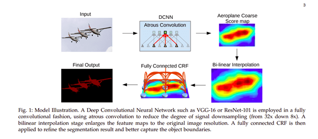
DeepLab

In this architecture, convolutions with upsampled filters are used for tasks that involve dense prediction. Segmentation of objects at multiple scales is done via atrous spatial pyramid pooling. Finally, DCNNs are used to improve the localization of object boundaries. Atrous convolution is achieved by upsampling the filters through the insertion of zeros or sparse sampling of input feature maps.

You can try its implementation on either PyTorch or TensorFlow.

Mask R-CNN

In this architecture, objects are classified and localized using a bounding box and semantic segmentation that classifies each pixel into a set of categories. Every region of interest gets a segmentation mask. A class label and a bounding box are produced as the final output. The architecture is an extension of the Faster R-CNN. The Faster R-CNN is made up of a deep convolutional network that proposes the regions and a detector that utilizes the regions.

Here is an image of the result obtained on the COCO test set.

Mask R-CNN results on the COCO test set — *Kaiming He et. al 2017 “Mask R-CNN” | Source*

Now, let’s work on a couple of Mask R-CNN use cases to automatically segment and construct pixel-wise masks for each object in an image.

Mask R-CNN use cases

For today’s introductory use case demonstration, we will be focusing on the Mask R-CNN framework for image segmentation. Specifically, we will utilize the weights of the Mask R-CNN model pretrained on the COCO dataset aforementioned to build an inference type of model.

During the model building process, we will also set up Neptune experiments to track and compare prediction performance with different hyperparameter tuning.

Now, let’s dive right in!

Install Mask R-CNN

First and foremost, we need to install the required packages and set up our environment. For this exercise, the algorithm implementation by Matterport will be used. Since there is no distributed version of this package so far, I put together several steps to install it by cloning from the Github repo:

One caveat here is that the original Matterport code has not been updated to be compatible with Tensorflow 2+. Hence, for all Tensorflow 2+ users, myself included, getting it to work becomes quite challenging as it would require significant modifications to the source code. If you prefer not to customize your code, an updated version for Tensorflow 2+ is also available here. Therefore, please make sure to clone the correct repo according to your Tensorflow versions.

Step 1: Clone the Mask R-CNN GitHub repo

Tensorflow 1+ and keras prior to 2.2.4:

git clone https://github.com/matterport/Mask_RCNN.git

Tensorflow 2+:

git clone https://github.com/akTwelve/Mask_RCNN.git updated_mask_rcnn

This will create a new folder named “updated_mask_rcnn” to differentiate the updated version from the original one.

Step 2:

Check and Install package dependencies
Navigate to the folder containing the repo
Run: pip install -r requirements.txt

Step 3:

Run setup to install the package
Run: python setup.py clean -all install

Few points to ponder:

If you encounter this error message: ZipImportError: bad local file header: mask_rcnn-2.1-py3.7.egg. then upgrade your setuptools.
For Windows users, if you are asked to install the pycocotools, be sure to use pip install pycocotools-windows, rather than the pycocotools as it may have compatibility issues with Windows.

Load the pretrained model

Next, from the Mask_RCNN project Github, let’s download the model weights into the current working directory: mask_rcnn_coco.h5

Image segmentation model tracking with Neptune

When it comes to the model training process, Neptune offers an effective yet easy-to-use way to track and log almost everything model-related, from hyperparameters specification to best model saving, to result from plots logging and so much more. What’s cool about experiment tracking with Neptune is that it will automatically generate performance charts for practitioners to compare different runs, and thus to select an optimal one.

For a more detailed explanation of configuring your Neptune environment and setting up your experiment, please check out this complete guide and my other blog here on Implementing macro F1 scores in Keras.

In this blog, I will also be demonstrating how to leverage Neptune during the image segmentation implementation. Yes, Neptune can well be used to track image processing models!

Importing all the required packages:

### Import packages
import neptune

import os
import sys
import numpy as np
import skimage.io
import matplotlib
import matplotlib.pyplot as plt
# Root directory of the project
ROOT_DIR = os.path.abspath(PATH_TO_YOUR_WORK_DIRECTORY) ## PATH_TO_YOUR_WORK_DIRECTORY

# Import Mask RCNN from the Github installation
sys.path.append(ROOT_DIR)  # To find local version
from mrcnn import utils
import mrcnn.model as modellib
from mrcnn import visualize
from mrcnn.config import Config
from mrcnn.model import MaskRCNN
from mrcnn.visualize import display_instances
from mrcnn.model import log

from keras.preprocessing.image import load_img
from keras.preprocessing.image import img_to_array
# Import COCO config for the dataset
sys.path.append(os.path.join(ROOT_DIR, "samples/coco/"))  # To find local version of coco
import coco

# Directory to save logs and trained model
MODEL_DIR = os.path.join(ROOT_DIR, "logs")

# Local path to your trained weights file
COCO_MODEL_PATH = os.path.join(ROOT_DIR, "mask_rcnn_coco.h5")

Now, let’s create a project with Neptune specifically for this image segmentation excise:

Next, in Python, creating a Neptune experiment connected to our Image Segmentation Project project, so that we can log and monitor the model information and outputs to Neptune:

import neptune
import os
# Connect your script to Neptune
myProject = 'YourUserName/YourProjectName'
project = neptune.init(api_token=os.getenv('NEPTUNE_API_TOKEN'),
                       project=myProject)
project.stop()

## How to track the weights and predictions in Neptune
npt_exp = neptune.init(
        api_token=os.getenv('NEPTUNE_API_TOKEN'),
        project=myProject,
        name='implement-MaskRCNN-Neptune',
        tags=['image segmentation', 'mask rcnn', 'keras', 'neptune'])

Few notes:

The api_token arg in the neptune.init() takes your Neptune API generated from the config steps;
The tags arg in the project.create_experiment() is optional, but it’s good to specify tags for a given project for easy sharing and tracking.

Having ImageSegmentationProject in my demo, along with its initial experiment successfully set up, we can move onto the modeling part.

Config the Mask R-CNN model

To run image segmentation and inference, we need to define our model as an instance of the Mask R-CNN class and construct a config object as one parameter fed into the class. The purpose of this config object is to specify how our model is leveraged to train and make predictions.

To warm-up, let’s only specify the batch size for the simplest implementation.

class InferenceConfig(coco.CocoConfig):
    GPU_COUNT = 1
    IMAGES_PER_GPU = 1

config = InferenceConfig()

### Sending log info to Neptune ###
npt_exp['Model Config Pars'] = str(config.to_dict())

Here, batch size = GPU_COUNT * IMAGES_PER_GPU, where both values are set to 1 as we will do segmentations on one image at a time. We also sent the config info to Neptune so that we can keep track of our experiments.

This video clip shows what we will see in our Neptune project, which I zoomed in to show details.

Image segmentation task # 1 with simple model configuration

With all the preparation work completed, we continue with the most exciting part — to make inferences on real images and see how the model is doing.

For task #1, we will work with this image, which can be downloaded here for free.

The following demonstrates how our Mask R-CNN model instance is defined:

# Create model object in inference mode.
model = modellib.MaskRCNN(mode="inference", model_dir=MODEL_DIR, config=config)

# Load weights trained on the COCO dataset 
model.load_weights(COCO_MODEL_PATH, by_name=True)

# Load the image for current task  
image_path = path_to_image_monks
img = load_img(image_path)
img = img_to_array(img)

# Make prediction
results = model.detect([img], verbose=1)

Points to ponder:

We specify the type of our current model to be “inference”, indicating that we are making image predictions/inference.
For the Mask R-CNN model to do prediction, the image must be converted to a Numpy array.
Rather than using model.predict() as we would for a Keras model prediction, we call the model.detect() function.

Sweet! Now we have the segmentation result, but how should we inspect the result and get a corresponding image out of it? Well, the model output is a dictionary containing multiple components,

ROIs: the regions-of-interest(ROI) for the segmented objects.
Masks: the masks for the segmented objects.
class_ids: the class ID integer for the segmented objects.
scores: the predicted probability of each segment belonging to a class.

To visualize the output, we can use the following code.

# get dictionary for first prediction
image_results = results[0]

box, mask, classID, score = image_results['rois'], image_results['masks'], image_results['class_ids'], image_results['scores']

# show photo with bounding boxes, masks, class labels and scores
fig_images, cur_ax = plt.subplots(figsize=(15, 15))
display_instances(img, box, mask, classID, class_names, score, ax=cur_ax)

# Log Predicted images to Neptune
npt_exp['Predicted Image'].upload(neptune.types.File.as_image(fig_images))

Here the class_names refers to a list of 80 object labels/categories in the COCO dataset. You can copy and paste it from my Github.

Running the code above returns this predicted output image in our Neptune experiment,

Impressive isn’t it! Our model successfully segmented the monks/humans and the dogs. What’s more impressive is that the model assigns a very high probability/confidence score (i.e., close to 1) to each segmentation!

Image segmentation task # 2 with model hyperparameter tuning

Now You may think that our model did a great job on the last image probably because every object is sort of at the focus, which makes the segmentation task easier because there weren’t too many confounding background objects. How about images with blurred backgrounds? Would the model achieve an equal level of performance?

Let’s experiment together.

Shown below is an image of an adorable teddy bear with a blurred background of cakes.

For better code organization, we can compile the aforementioned model inference steps into a function runMaskRCNN, which takes in two primary args.: modelConfig and imagePath:

def runMaskRCNN(modelConfig, imagePath, MODEL_DIR=MODEL_DIR, COCO_MODEL_PATH=COCO_MODEL_PATH):
    '''
    Args:
        modelConfig: config object
        imagePath: full path to the image
   '''

    model = modellib.MaskRCNN(mode="inference", model_dir=MODEL_DIR, config=modelConfig)
    model.load_weights(COCO_MODEL_PATH, by_name=True)

    image_path = imagePath
    img = load_img(image_path)
    img = img_to_array(img)

    results = model.detect([img], verbose=1)
    modelOutput = results[0]

    return modelOutput, img

Experimenting with the first model, we are using the same config as for task #1. This information will be sent to Neptune for tracking and comparing later.

cur_image_path = path_to_image_teddybear
image_results, img = runMaskRCNN(modelConfig=config, imagePath=cur_image_path)

# Log model config parameters to Neptune
npt_exp['Model Config Pars'] = str(config.to_dict())
fig_images, cur_ax = plt.subplots(figsize=(15, 15))
display_instances(img, image_results['rois'], image_results['masks'], image_results['class_ids'], class_names, image_results['scores'], ax=cur_ax)

# Log Predicted images to Neptune
npt_exp['Predicted Image'].upload(neptune.types.File.as_image(fig_images))

Predicted by this model, the following output image should show up in our Neptune experiment log.

As we can see, the model successfully segmented the teddy bear and cupcakes in the background. As far as the cupcake cover goes, the model labeled it as “bottle” with a fairly high probability/confidence score, the same applies to the cupcake tray underneath, which was identified as “bowl”. Both make sense!

Overall, our model did a decent job identifying each object. However, we do also notice that a part of the cake was mislabeled as “teddy bear” with a probability score of 0.702 (i.e., the green box in the middle).

How can we fix this?

Customize the config object for model hyperparameter tuning

We can construct a custom model config to override the hyperparameters in the base config class. Hence to tailor the modeling process specifically for this teddy bear image:

class CustomConfig(coco.CocoConfig):
    """Configuration for inference on the teddybear image.
    Derives from the base Config class and overrides values specific
    to the teddybear image.
    """
    # configuration name
    NAME = "customized"
    # number of classes: +1 for background
    NUM_CLASSES = 1 + 80

    # batch size = 1 for one image
    GPU_COUNT = 1
    IMAGES_PER_GPU = 1

    # how many steps in one epoch
    STEPS_PER_EPOCH = 500
    # min. probability for segmentation
    DETECTION_MIN_CONFIDENCE = 0.71

    # learning rate, momentum and weight decay for regularization
    LEARNING_RATE = 0.06
    LEARNING_MOMENTUM = 0.7
    WEIGHT_DECAY = 0.0002

    VALIDATION_STEPS = 30

config = CustomConfig()

## Log current config to Neptune
npt_exp.send_text('Model Config Pars', str(config.to_dict()))

After running the model with this new config, we will see this image with correct segmentations in the Neptune project log,

In our custom config class, we specified the number of classes, steps in each epoch, learning rate, weight decay, and so on. For a complete list of hyperparameters, please refer to the config.py file in the package.

We encourage you to play around with different (hyperparameter) combinations and set up your Neptune project to track and compare their performance. The video clip below showcases the two models we just built along with their prediction results in Neptune.

Mask R-CNN layer weights

For the geeky audience out there who want to go deep into the weeds with our model, we can also collect and visualize the weights and biases for each layer of this CNN model. The following code snippet demonstrates how to do this for the first 5 convolutional layers.

### Show model weights and biases 
LAYER_TYPES = ['Conv2D']
# Get layers
layers = model.get_trainable_layers()
layers = list(filter(lambda l: l.__class__.__name__ in LAYER_TYPES, layers))
print(f'Total layers = {len(layers)}')

## Select a subset of layers
layers = layers[:5]

# Display Histograms
fig, ax = plt.subplots(len(layers), 2, figsize=(10, 3*len(layers)+10),
                       gridspec_kw={"hspace":1})

for l, layer in enumerate(layers):
    weights = layer.get_weights()
    for w, weight in enumerate(weights):
        tensor = layer.weights[w]
        ax[l, w].set_title(tensor.name)
        _ = ax[l, w].hist(weight[w].flatten(), 50)

### Log information to Neptune
npt_exp['Model_Weights'].upload(neptune.types.File.as_image(fig))
### Stop the run after logging
npt_exp.stop()

This is a screenshot of what displays in Neptune, showing the histogram of layer weights,

Image segmentation loss functions

Semantic segmentation models usually use a simple cross-categorical entropy loss function during training. However, if you are interested in getting the granular information of an image, then you have to revert to slightly more advanced loss functions.

Let’s go through a couple of them.

Focal Loss

This loss is an improvement to the standard cross-entropy criterion. This is done by changing its shape such that the loss assigned to well-classified examples is down-weighted. Ultimately, this ensures that there is no class imbalance. In this loss function, the cross-entropy loss is scaled with the scaling factors decaying at zero as the confidence in the correct classes increases. The scaling factor automatically down weights the contribution of easy examples at training time and focuses on the hard ones.

Dice loss

This loss is obtained by calculating smooth dice coefficient function. This loss is the most commonly used loss is segmentation problems.

Intersection over Union (IoU)-balanced Loss

The IoU-balanced classification loss aims at increasing the gradient of samples with high IoU and decreasing the gradient of samples with low IoU. In this way, the localization accuracy of machine learning models is increased.

Boundary loss

One variant of the boundary loss is applied to tasks with highly unbalanced segmentations. This loss’s form is that of a distance metric on space contours and not regions. In this manner, it tackles the problem posed by regional losses for highly imbalanced segmentation tasks.

Weighted cross-entropy

In one variant of cross-entropy, all positive examples are weighted by a certain coefficient. It is used in scenarios that involve class imbalance.

Lovász-Softmax loss

This loss performs direct optimization of the mean intersection-over-union loss in neural networks based on the convex Lovasz extension of sub-modular losses.

Other losses worth mentioning are:

TopK loss whose aim is to ensure that networks concentrate on hard samples during the training process.
Distance penalized CE loss that directs the network to boundary regions that are hard to segment.
Sensitivity-Specificity (SS) loss that computes the weighted sum of the mean squared difference of specificity and sensitivity.
Hausdorff distance(HD) loss that estimated the Hausdorff distance from a convolutional neural network.

These are just a couple of loss functions used in image segmentation. To explore many more check out this repo.

Image segmentation datasets

If you are still here, chances are that you might be asking yourself where you can get some datasets to get started.

Let’s look at a few.

1. Common Objects in COntext — Coco Dataset

COCO is a large-scale object detection, segmentation, and captioning dataset. The dataset contains 91 classes. It has 250,000 people with key points. Its download size is 37.57 GiB. It contains 80 object categories. It is available under the Apache 2.0 License and can be downloaded from here.

2. PASCAL Visual Object Classes (PASCAL VOC)

PASCAL has 9963 images with 20 different classes. The training/validation set is a 2GB tar file. The dataset can be downloaded from the official website.

3. The Cityscapes Dataset

This dataset contains images of city scenes. It can be used to evaluate the performance of vision algorithms in urban scenarios. The dataset can be downloaded from here.

4. The Cambridge-driving Labeled Video Database — CamVid

This is a motion-based segmentation and recognition dataset. It contains 32 semantic classes. This link contains further explanations and download links to the dataset.

Image segmentation frameworks

Now that you are armed with possible datasets, let’s mention a few tools/frameworks that you can use to get started.

FastAI library — given an image this library is able to create a mask of the objects in the image.
Sefexa Image Segmentation Tool — Sefexa is a free tool that can be used for Semi-automatic image segmentation, analysis of images, and creation of ground truth
Deepmask — Deepmask by Facebook Research is a Torch implementation of DeepMask and SharpMask
MultiPath — This a Torch implementation of the object detection network from “A MultiPath Network for Object Detection”.
OpenCV — This is an open-source computer vision library with over 2500 optimized algorithms.
MIScnn — is a medical image segmentation open-source library. It allows setting up pipelines with state-of-the-art convolutional neural networks and deep learning models in a few lines of code.
Fritz: Fritz offers several computer vision tools including image segmentation tools for mobile devices.

Final thoughts

Hopefully, this article gave you some background into image segmentation as well as some tools and frameworks. We also hope that the use case demonstration could spark your interest in getting started exploring this fascinating area of deep neural networks

We’ve covered:

what image segmentation is,
a couple of image segmentation architectures,
some image segmentation losses,
image segmentation tools and frameworks,
use case implementation with the Mask R-CNN algorithm.

For more information check out the links attached to each of the architectures and frameworks. In addition, the Neptune project is made available here, and the full code can be accessed at this Github repo here.

Happy segmenting!